
Making realistic 3D topographic maps in R
May 25, 2022 | Milos Popovic
In one of my previous tutorials I’ve showed you how to make crisp topographic maps programatically in R using a few lines of code.
This time I will demonstrate how to create realistic 3D topographic maps using satellite imagery as an overlay map 😮. We will first crop the elevation data to the extent of Austria, download the satellite imagery and overlay the map, and turn everything into a 3D plot.
Are you ready to rumble?
Import libraries
We’ll load several essential packages such as tidyverse and sf for spatial analysis and data wrangling; giscoR for importing the shapefile of Austria; elevatr for downloading raster data; as well as rayshader for making a 3D map, which we have already used here.
Since we’ll import the satellite data using POST request we will call to rescue httr and jsonlite. Finally, we will use png to load the satellite image into R.
libs <- c("elevatr", "rayshader", "tidyverse",
	"sf", "giscoR", "jsonlite", "httr", "png")

installed_libs <- libs %in% rownames(installed.packages())
if (any(installed_libs == F)) {
  install.packages(libs[!installed_libs])
}

invisible(lapply(libs, library, character.only = T))
Fetch the shapefile of Austria
Because we aim to produce a topographic map of Austria we first import the country’s shapefile using giscoR. We will stick to a rather low resolution in order to speed up the raster cropping phase. Also, we transform the sf object to a WGS84 projection before venturing forth.
# 1. GET COUNTRY MAP
#-------------------

crsLONGLAT <- "+proj=longlat +datum=WGS84 +no_defs"

get_country_sf <- function(country_sf, country_transformed) {

	country_sf <- giscoR::gisco_get_countries(
    	year = "2016",
    	epsg = "4326",
    	resolution = "10",
    	country = "Austria")

	country_transformed <- st_transform(country_sf, crs = crsLONGLAT)

	return(country_transformed)
}

austria_transformed <- get_country_sf()
Import topographic data
In the following step, we call elevatr to arms. We read the topographic data from a server and crop the raster to the shapefile of Austria. If your session crashes at this point, please feel free to decrease the z value. In the last step, we use raster_to_matrix to turn our raster into a matrix so that it can be processed by rayshader.
# 2. GET ELEVATION DATA
#----------------------

get_elevation_data <- function(country_elevation, country_elevation_df) {

	country_elevation <- get_elev_raster(
		locations = austria_transformed,
		z = 7,
		clip = "locations")

	elevation_mat <- raster_to_matrix(country_elevation)

	return(elevation_mat)
}

austria_dem <- get_elevation_data()
Notice the dimensions of the matrix below: we will pass the augmented values to the image save function at the very end. For now, let’s store the height and width.
Mosaicing & Projecting
Clipping DEM to locations
Note: Elevation units are in meters.
Error in (function (x)  : attempt to apply non-function
Error in (function (x)  : attempt to apply non-function
Error in (function (x)  : attempt to apply non-function
[1] "Dimensions of matrix are: 537x1552"

h <- 537
w <- 1552
Retrieve overlay satellite imagery
In this tutorial, we will create a realistic 3D topographic map of Austria. This means that we will use true colors from the existing satellite imagery rather than a customized color palette.
To do so, we will query data from ArcGIS REST API, which offers an open and straightforward web interface to communicate with ArcGIS Server. All the satellite imagery is accessible through URLs for any given services and takes place via the interface.
This requires us to build a POST request similar to what we did here. We compile a request message to the server, in which we define what is requested and the content of the request.
Below, we make a POST request by calling the ArcGIS REST page and compiling a message with a web form. For our form submission, we define several map parameters in the form of a list (you can find the detailed instructions here). These are as follows:
- baseMap, which includes the location of the base map layers from the World_Imagery directory;
- exportOptions, the size of the image that should be downloaded from the server denoted by height/width;
- mapOptions, the coordinate reference system that should be used (crs_bb) and the bounding box parameters.
Then we issue a GET call to the designated url and declare that the response returns a JSON object, the PNG format for the map image, default MAP_ONLY layout that contains no additional graphics such as legends, scale bar, etc, and wrap our parameters into JSON format. For clarity’s sake, you can find the thorough guidelines here.
# 3. GET OVERLAY SATELLITE IMAGE
#----------------------

bb <- st_bbox(austria_transformed)
type <- "World_Imagery"
file <- NULL
height <- h*6
width <- w*6
crs_bb <- 4326

get_satellite_img <- function(url, params, res) {

  url <- parse_url("https://utility.arcgisonline.com/arcgis/rest/services/Utilities/PrintingTools/GPServer/Export%20Web%20Map%20Task/execute")

  params <- list(
    baseMap = list(
      baseMapLayers = list(
        list(url = unbox("https://services.arcgisonline.com/ArcGIS/rest/services/World_Imagery/MapServer"))
      )
    ),
    exportOptions = list(
      outputSize = c(width, height)
    ),
    mapOptions = list(
      extent = list(
        spatialReference = list(wkid = unbox(crs_bb)),
        xmax = unbox(bb["xmax"]),
        xmin = unbox(bb["xmin"]),
        ymax = unbox(bb["ymax"]),
        ymin = unbox(bb["ymin"])
      )
    )
  )

  res <- GET(
    url,
    query = list(
      f = "json",
      Format = "PNG32",
      Layout_Template = "MAP_ONLY",
      Web_Map_as_JSON = toJSON(params))
  )

	return(res)

}

res <- get_satellite_img()
We retrieve the results in the form of list and issue another GET call to extract the image values from the list. Then we pull out the image and save it on our local drive. Don’t worry about the image size, it’s slightly over 65 MB!
write_map_png <- function(res_body, img_res, img_bin, file) {

	res_body <- content(res, type = "application/json")
	img_res <- GET(res_body$results[[1]]$value$url)
	img_bin <- content(img_res, "raw")
	file <- paste0(getwd(), "/austria_image.png")
	writeBin(img_bin, file)
}

write_map_png()
In the final step, we load the image into R using readPNG.
get_map_png <- function(img_file, austria_img) {

	img_file <- "austria_image.png"
	austria_img <- readPNG(img_file)

	return(austria_img)
}

austria_img <- get_map_png()
3D topographic map of Austria
Alright, we are all set to produce our 3D map 🥁!
In this section we solely rely on rayshader for image rendering. First, we define a base layer using sphere_shade(texture =“desert”). Then we pass the overlay image and declare that this layer will have the highest visibility with alphalayer = .99.
Finally, we issue a call to produce the 3D map using the matrix data. We set a few parameters such as zscale, where lower zscale values exaggerate elevation features, and zoom, which defines the zoom factor. For the window size we use the aforementioned matrix dimensions. If you are interested in these and additional features of plot_3d, then have a look at the detailed guidelines on this page.
# 4. 3D MAP
#---------
austria_dem %>%
sphere_shade(texture ="desert") %>%
add_overlay(austria_img, alphalayer = .99) %>%
plot_3d(austria_dem,
zscale = 15,
fov = 0,
theta = 0,
zoom = .55,
phi = 75,
windowsize = c(1552, 537),
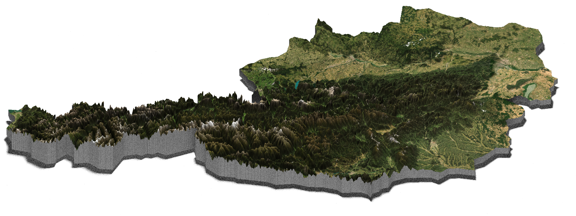
background="black")Here is the pre-rendered, 2D version of the map 🧐.

Last but not least we will render the image and turn it into a 3D beauty. Apart from defining the file name, we also pass a very high intensity of the scene light with a 90 degree angle. You may want to check other rendering and styling options for renderhighquality function <a href=”https://www.rayshader.com/reference/renderhighquality.html” target=“_blank” rel=“noopener noreferrer”>here. We wrap this up with pre-defined width and height values multiplied by 3 to get a high resolution plot.
render_highquality(filename="austria_dem.png",
	lightintensity=1500,
	lightaltitude=90,
  title_text="Topography of AUSTRIA\n©2022 Milos Popovic https://milospopovic.net",
  title_font="Georgia",
  title_color="grey20",
  title_size=100,
  title_offset=c(360,180),
	width=w*3,
	height=h*3)
Aaaaand, here is the final map! 😍

Alright, that’s all ladies and gents! In this tutorial, you learned how to load satellite imagery using POST call and create a 3D topographic map. And all this was achieved in R! Feel free to check the full code here, clone the repo and reproduce, reuse and modify the code as you see fit.
Following this tutorial only the sky is the limit. You can tweak my code a bit to create a myriad of 3D elevation maps for any country in the world.
I’d be happy to hear your view on how this map could be improved or extended to other geographic realms. To do so, please follow me on Twitter, Instagram or Facebook! Also, feel free to support my work by buying me a coffee here!