
Web scrapping SIPRI arms data using search request with R
March 06, 2022 | Milos Popovic
Did you know that the UN Security Council permanent members controlled nearly 90% of the arms market in 2008–2016 and that the United States alone accounted for more than 40% of all arms sales globally 😲? Arms sales bring big bucks but it’s not only about the money.
In fact, research in political science has shown that arms sales are one of the most potent foreign policy weapons in the arsenal of major powers. Major powers can use arms transfers to influence foreign policies of their client states, balance against their rival’s influence, or impose outright hegemony on the state importer.
The United States was particularly successful at influencing their clients’ foreign policy through arms sales during the Cold War while the Soviet Union ensured that their arms importers align with Soviet objectives in the Middle East and Africa. Even after the Cold War, Russia used its close military ties with Nicaragua, Syria and Venezuela to secure their recognition of Abkhazia and South Ossetia, while NATO members, the Gulf States, Turkey and Colombia have recognized Kosovo, in accord with American preferences.
In this tutorial, we’ll analyze American arms transfer to Europe in the last 5 years using the Stockholm Institute for Peace Research’s (SIPRI) Arms Transfers Database to measure arms transfers. SIPRI measures arms transfers as the number of weapon systems or subsystems delivered/produced in a given year to the country’s government under contract, including small arms, tanks, artillery, anti-missile systems, satellites and warplanes.
If you ever used this database, you know how big pain in the ass is to retrieve a table in a decent format. Basically, if you manually fill in the required fields and submit your query the output excel file will be in the form of a report with some descriptive text and a table in the middle of the sheet. Ouch 😭.
Not so long ago I bumped into an elegant solution in this blog post using web scrapping with post request in non-R setting. Essentially, to get the data, we would submit a web request, and retrieve and format the data. Unlike the GET request that asks the SIPRI server to return the arms data, a POST request asks the server to accept a completed web form with a list of items we need. In this tutorial, I want to show you how to do this in R!
Request data
We kick off our journey by loading several important libraries such as rvest, which allows us to scrape data from web pages by sending a POST request to the server; httr for retreiving the data using GET function; tidyverse and sf for spatial analysis; giscoR for the spatial file of Europe; and cartogram library will help us map arms data in the form of non-contiguous cartogram.
windowsFonts(georg = windowsFont('Georgia'))

libs <- c("rvest", "httr", "tidyverse", "sf", "giscoR", "cartogram")

installed_libs <- libs %in% rownames(installed.packages())
if (any(installed_libs == F)) {
  install.packages(libs[!installed_libs])
}

invisible(lapply(libs, library, character.only = T))
At the very outset, we compile a request message to the server. The request message is composed of the request line (what is requested), headers (who is sending and what) and body (the content of the request). Below, we submit the form on SIPRI’s arms transfer page. We make a POST request by calling this page and compiling a message with a web form. For our form submission, we include a list of items such as first and last year and export from the United States by partner country. Finally, we read the data from the html source and store it into a list object.
get_data <- function(url, res, r) {

  url <- "https://armstrade.sipri.org/armstrade/html/export_values.php"

  res <- POST(
    url = url,
    encode = "form",
    body = list(
      `low_year` = '2016',
      `high_year` = '2020',
      `import_or_export` = 'export',
      `country_code` = 'USA',
      `summarize` = 'country',
      `filetype` = 'html'
    ),
    verbose()
  )

  r <- res %>%
    read_html() %>%
    html_table()

return(r)
}
Data formatting
Now is the time to get our hands dirty with data formatting. The data that we just retrieved is a list object with two components. We need to identify the component that contains info on arms. Judging by the looks of it, this could be the second component because it includes the verbose part of the SIPRI arms database and a bunch of other values.
df <- get_data()
str(df)

List of 4
 $ : tibble [2 x 3] (S3: tbl_df/tbl/data.frame)
  ..$ X1: logi [1:2] NA NA
  ..$ X2: logi [1:2] NA NA
  ..$ X3: chr [1:2] NA "The independent resource on global security"
 $ : tibble [113 x 8] (S3: tbl_df/tbl/data.frame)
  ..$ X1: chr [1:113] "TIV of arms exports from United States, 2016-2020" "Figures are SIPRI Trend Indicator Values (TIVs) expressed in millions." "Figures may not add up due to the conventions of rounding." "A '0' indicates that the value of deliveries is less than 0.5m" ...
  ..$ X2: chr [1:113] "TIV of arms exports from United States, 2016-2020" "Figures are SIPRI Trend Indicator Values (TIVs) expressed in millions." "Figures may not add up due to the conventions of rounding." "A '0' indicates that the value of deliveries is less than 0.5m" ...
  ..$ X3: chr [1:113] "TIV of arms exports from United States, 2016-2020" "Figures are SIPRI Trend Indicator Values (TIVs) expressed in millions." "Figures may not add up due to the conventions of rounding." "A '0' indicates that the value of deliveries is less than 0.5m" ...
Spot on! 🥳 The code below extracts the table from the list, converts it into a data frame and tranposes the table.
d <- df[[2]] %>%
      as_tibble() %>% # convert to data.frame
      t()
 head(d)

 [,1]
X1 "TIV of arms exports from United States, 2016-2020"
X2 "TIV of arms exports from United States, 2016-2020"
X3 "TIV of arms exports from United States, 2016-2020"
X4 "TIV of arms exports from United States, 2016-2020"
X5 "TIV of arms exports from United States, 2016-2020"
X6 "TIV of arms exports from United States, 2016-2020"
The resulting table has a plethora of columns, some of which are merely a description of the queried table. Since we only need partners and their total imports from the United States, we get rid of excess information in the chunk below. First, we delete the verbose columns, including the last two columns. Then we declare the first row to be header using colnames(d) <- as.character(d[1,]). Finally, we get rid of the first row and rename the first column to year.
d <- d[,-c(1:10, (ncol(d)-1):ncol(d))]
colnames(d) <- as.character(d[1,])
d <- d[-1,] %>%
as.data.frame()
names(d)[1] <- "year"
head(d)
year Afghanistan Albania Algeria Angola Argentina Australia Austria Bahrain
X2 2016 72   19   6 889    
X3 2017 251 4   2 34 947   20
X4 2018 320 2 3   10 907   7
X5 2019 368 5     11 1004 1 2
X6 2020 227       7 1132    
X7 Total 1238 11 22 2 68 4880 1 28
Now we are only interested in total arms imports from the United States for the period 2016-2020. So, we only need the Total row.
d <- d[d$year == "Total", ]
head(d)

 year Afghanistan Albania Algeria Angola Argentina Australia Austria Bahrain
X7 Total        1238      11      22      2        68      4880       1      28
NA  <NA>        <NA>    <NA>    <NA>   <NA>      <NA>      <NA>    <NA>    <NA>
We have two rows, one with values and another with missing values in the wide format. We need to get rid of the NAs and reshape our table into a long format. The chunk below does that for us 🤓!
d <- d %>%
         filter_all(any_vars(!is.na(.))) %>% #only complete rows
         gather(country, value, -year) %>% #reshape
         select(country, value) %>% #select only country and value
         mutate(value = as.numeric(value))
head(d)

country value
1 Afghanistan  1238
2     Albania    11
3     Algeria    22
4      Angola     2
5   Argentina    68
6   Australia  4880
Here is the entire code from this section.
clean_data <- function(df, d) {

  df <- get_data() # call list
  d <- df[[2]] %>% #extract table from the list
      as_tibble() %>% # convert to data.frame
      t() #transpose
  d <- d[,-c(1:10, (ncol(d)-1):ncol(d))] #get rid of descriptive/empty columns
  colnames(d) <- as.character(d[1,]) # replace header with first row
  d <- d[-1,] %>%
    as.data.frame()
  names(d)[1] <- "year" #label year column
  d <- d[d$year == "Total", ]  #filter Total values for the period
  d <- d %>%
         filter_all(any_vars(!is.na(.))) %>% #only complete rows
         gather(country, value, -year) %>% #reshape
         select(country, value) %>% #select only country and value
         mutate(value = as.numeric(value)) # declare value to be numeric

  return(d)
}
Fetch Europe sf object
We came a long way from the POST request and cleaning up the messy list and turning it into a usable data frame.
In this tutorial, we’ll make a map of Europe, so let’s filter the European countries using a trick from this tutorial. Ah, and we also correct the names for Bosnia and UK to be able to merge it with the arms data later on.
europeList <- function(urlfile, iso3) {
  urlfile <-'https://raw.githubusercontent.com/lukes/ISO-3166-Countries-with-Regional-Codes/master/all/all.csv'

  iso3 <- read.csv(urlfile) %>%
        filter(region=="Europe") %>%
        select("name", "alpha.3") %>%
        rename(iso3 = alpha.3,
               country = name) %>%
        mutate(country = replace(country, str_detect(country, "Bosnia and Herzegovina"), "Bosnia-Herzegovina")) %>%
        mutate(country = replace(country, str_detect(country, "United Kingdom of Great Britain and Northern Ireland"), "United Kingdom"))
  return(iso3)
}

countries <- europeList()
Then, we call giscoR to get the spatial object of Europe and filter countries from the abovementioned list.
europeMap <- function(europe, eur) {

  europe <- giscoR::gisco_get_countries(
  year = "2016",
  epsg = "4326",
  resolution = "10",
  region = "Europe"
) %>%
  rename(iso3 = ISO3_CODE)

eur <- europe %>% dplyr::filter(iso3%in%countries$iso3)
return(eur)
}
Join arms data and Europe sf object
To join arms data and Europe sf object, we first need to filter European countries and retrieve the ISO3 code from list of European countries. The chunk below takes care of that.
europeArmsData <- function(arms, l) {

l <- europeList()

arms <- clean_data() %>%
  right_join(l, "country") %>%
  filter_all(any_vars(!is.na(.)))

return(arms)
}
Now we can join the arms data and the sf object on iso3 field and select country name, value and geometry columns.
joinArmsData <- function(armsDF, eurSF, arms) {

armsDF <- europeArmsData()
eurSF <- europeMap()

arms <- eurSF %>%
  left_join(armsDF, "iso3") %>%
  select(country, value, geometry)

return(arms)
}

f <- joinArmsData()
And here it is! We are ready for the cartogram map 😎.
head(f)

Simple feature collection with 6 features and 2 fields
Geometry type: MULTIPOLYGON
Dimension:     XY
Bounding box:  xmin: 1.44257 ymin: 39.64851 xmax: 21.05607 ymax: 51.50246
Geodetic CRS:  WGS 84
             country value                       geometry
1            Andorra    NA MULTIPOLYGON (((1.75495 42....
2            Albania    11 MULTIPOLYGON (((20.02705 42...
3            Austria     1 MULTIPOLYGON (((16.88406 48...
4        Switzerland    92 MULTIPOLYGON (((9.4956 47.5...
5 Bosnia-Herzegovina     2 MULTIPOLYGON (((18.839 44.8...
6            Belgium    17 MULTIPOLYGON (((5.89207 50....
Non-contiguous cartogram map
In this tutorial, we’ll map our arms data using the non-contiguous cartogram. This is a mapping technique that scales geographic units to show relative differences in quantitative values. While every unit is resized based on the input values, the shapes are not displaced but not distorted. In our case, we will resize European countries base on their arms imports from the United States.
Although some may struggle with scaling and displacement of the countries, the advantage of this approach is the display of relative sizes without normalization of our data.
Library cartogram offers an elegant cartogram_ncont function to compute parameters for our cartogram. But, to use this function we first need to project our sf object. We also need to set several parameters such as weight and inplace=F. The latter makes sure that the new polygons are created over every polygon in a multipolygon. For example, this will create the polygon of France over mainland France and Corsica, respectively. If we didn’t use this parameter, then we would have a single scaled polygon of France somewhere in Spain 😬.
crsLAEA <- "+proj=laea +lat_0=52 +lon_0=10 +x_0=4321000 +y_0=3210000 +datum=WGS84 +units=m +no_defs"

getNonCartogram <- function(f, nc) {

  f <- joinArmsData() %>%
        st_transform(crs = crsLAEA)
  nc <- cartogram_ncont(f,
                  weight = "value",
                  inplace=F)
return(nc)
}
Mapping
We’ll limit the view of our map via a bounding box. Let’s create a bounding box and reproject the coordinates to Lambert projection. First, we define the WGS84 projection as crsLONGLAT. Next, we run st_sfc to create a bounding box conveniently labeled bb with the latitude and longitude coordinates under the WGS84 definition. Finally, we transform bb into the Lambert projection using st_transform and make a bounding box b with reprojected coordinates by running st_bbox(laeabb).
crsLONGLAT <- "+proj=longlat +datum=WGS84 +no_defs"

bbox <- function(bb, laeabb, b) {

bb <- st_sfc(
  st_polygon(list(cbind(
    c(-10.6600, 33.00, 33.00, -10.6600, -10.6600),
    c(32.5000, 32.5000, 71.0500, 71.0500, 32.5000)
    ))),
  crs = crsLONGLAT)

laeabb <- st_transform(bb, crs = crsLAEA)
box <- st_bbox(laeabb)
return(box)
}
It’s time to map, folks! In the chunk below, we use the standard template for map-making that you encountered in my previous tutorials. One additional feature is rmapshaper::ms_erase, which will return the non-overlapping difference of the Europe and cartogram polygons. We apply this trick in order to avoid using transparent background in our Europe map.
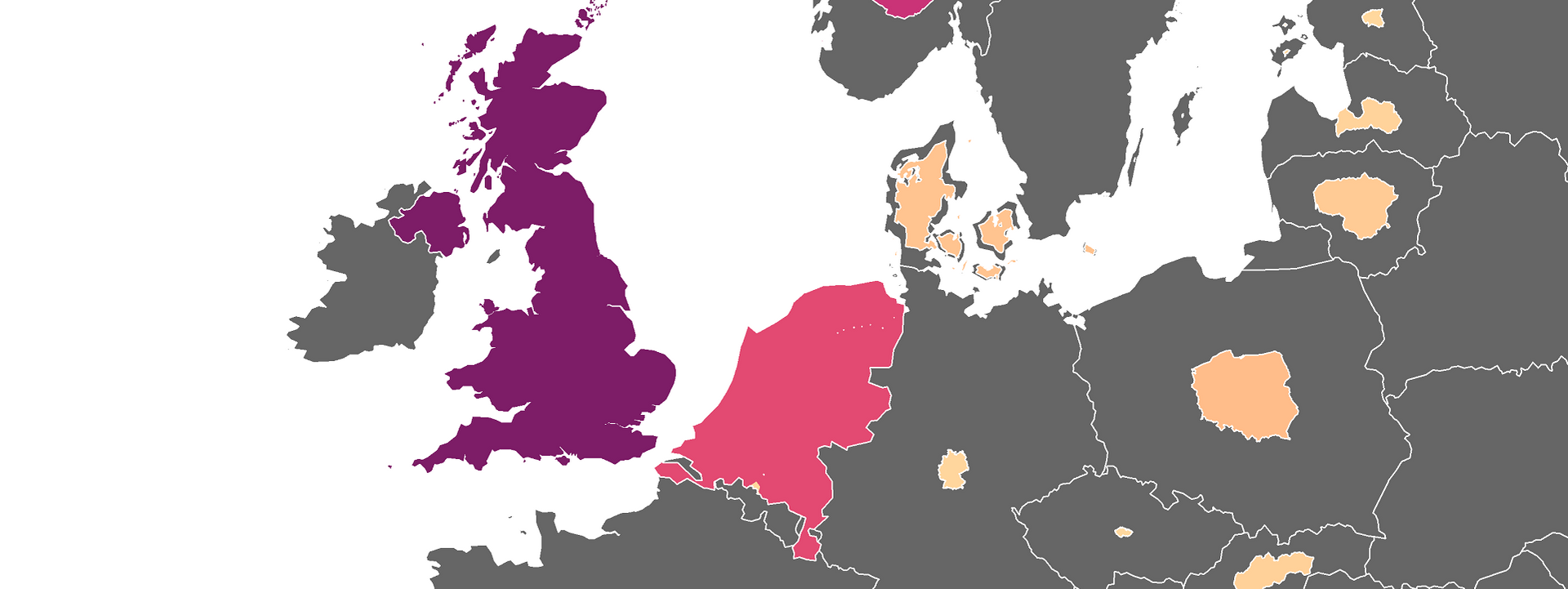
armsMap <- function(nc, eur, b, p) {

  nc <- getNonCartogram()
  eur <- europeMap() %>% st_transform(crs = crsLAEA)
  e <- rmapshaper::ms_erase(eur, nc)
  b <- bbox()

  p <-
  ggplot(nc) +
  geom_sf(aes(fill = value), color = NA) +
  geom_sf(data=e, fill="grey40", color="white", size=0.2) +
  coord_sf(crs = crsLAEA,
      xlim = c(b["xmin"], b["xmax"]),
      ylim = c(b["ymin"], b["ymax"])) +
  scale_fill_gradientn(
    name = "quantity",
    colours = hcl.colors(n = 5, "SunsetDark", rev = T),
    limits = c(min(nc$value), max(nc$value)),
    n.breaks = 8) +
  guides(fill=guide_legend(
      direction = "horizontal",
      keyheight = unit(1.15, units = "mm"),
      keywidth = unit(15, units = "mm"),
      title.position = 'top',
      title.hjust = 0.5,
      label.hjust = .5,
      nrow =1,
      byrow = T,
      reverse = F,
      label.position = "bottom")
    ) +
  theme_minimal() +
    theme(text = element_text(family = "georg"),
      panel.background = element_blank(),
      legend.background = element_blank(),
      legend.position = c(.45, .05),
      panel.border = element_blank(),
      panel.grid.minor = element_blank(),
      panel.grid.major = element_blank(),
      plot.title = element_text(size=14, color="#60047a", hjust=0.5, vjust=1),
      plot.caption = element_text(size=8, color="grey60", hjust=.5, vjust=10),
      axis.title.x = element_text(size=10, color="grey20", hjust=0.5, vjust=0),
      legend.text = element_text(size=9, color="grey20"),
      legend.title = element_text(size=11, color="grey20"),
      strip.text = element_text(size=12),
      plot.margin = unit(c(t=1, r=-2, b=-1, l=-2),"lines"),
      axis.title.y = element_blank(),
      axis.ticks = element_blank(),
      axis.text.x = element_blank(),
      axis.text.y = element_blank()) +
  labs(y="",
      subtitle="",
      x = "",
      title="US Arms Sales (2016-2020)",
      caption="©2022 Milos Popovic https://milospopovic.net\nSource: SIPRI Arms Transfers Database, https://sipri.org/databases/armstransfers")
return(p)
}

map <- armsMap()
ggsave(filename="sipri.png", width=7, height=8.5, dpi = 600, device='png', map)
You’ll notice that NATO countries bought arms from the United States but only a handful of countries imported a considerable amount of arms from the United States (Netherlands being one of the most visible ones!).

In this tutorial, I showed you how to use POST request to fetch arms sales data, clean it up, and make a cool non-contiguous cartogram. You could apply this project to other databases out there and a few come to mind such as, for example, The UN Comtrade database.
Feel free to check the full code here, clone the repo and reproduce, reuse and modify the code as you see fit.
I’d be happy to hear your view on how this map could be improved or extended to other geographic realms. To do so, please follow me on Twitter, Instagram or Facebook.