
3D maps with sf and ggplot2 in R
May 01, 2022 | Milos Popovic
I’ve played a bit with 3D mapping in R, which gave birth to this map of average forest height in Brazil 🌳.
In this tutorial, we will create a similar 3D map, using more recent Global Land Analysis & Discovery (GLAD) data on forest cover height. The GLAD dataset is derived from the NASA Global Ecosystem Dynamics Investigation (GEDI) lidar footprint-based measurement of forest canopy height and Landsat time-series data using a supervised machine learning technique. The GLAD team at the University of Maryland applied machine learning to the NASA/Landsat integrated dataset to improve forest height modeling accuracy. If you are interested in further details about the 2019 GLAD Global Forest Canopy Height dataset as well as the known issues related to GEDI data quality, I encourage you to have a look at the dedicated website.
Our main aim is to fetch the raster data on forest height, compute average forest height over a hexagonal map of Brazil, and turn a ggplot2 flat map into a 3D map.
Now, let’s dig into the data, shall we? 🧐
Import libraries
We’ll load a few important libraries, including several standard culprits such as tidyverse and sf for spatial analysis and data wrangling; giscoR for importing the shapefile of Brazil; classInt for creating bins; and exactextractr for zonal statistics, which we have already used here and here.
There’s a couple of novices among the imported libraries: we will use terra to import the forest data in raster format without downloading it; also, we will import rayshader to make a 3D map of forest height in Brazil!
#install dev version of terra package
install.packages('terra', repos='https://rspatial.r-universe.dev')

# libraries we need
libs <- c("rayshader", "tidyverse", "sf",
  "classInt", "giscoR", "terra", "exactextractr")

# install missing libraries
installed_libs <- libs %in% rownames(installed.packages())
if (any(installed_libs == F)) {
  install.packages(libs[!installed_libs])
}

# load libraries
invisible(lapply(libs, library, character.only = T))

# define longlat CRS
crsLONGLAT <- "+proj=longlat +datum=WGS84 +no_defs"
Create a hexagonal map of Brazil
We will divide the shapefile of Brazil into hexagonal fields the size of approximately 30,000 m² each. This step is necessary to make sure that we capture equal area size in computing forest height. Eventually we will turn those hex fields into 3D bars.
Using giscoR we first obtain the shapefile of Brazil and then transform it from a degree into a metric projection. Otherwise we wouldn’t know the size of hex fields in m². Then we create a hex grid of roughly 30,000 m² each using the formula for the hexagonal area size, which is
where s is side length and is equal to 107 meters. Note that we use st_intersection to clip the grid to the polygon area of Brazil so that hex cells overlapping the borders are cut off. This will make the bordering hex fields somewhat smaller. Finally, we keep only (multi)polygonal features and transform the hex shapefile into a EPSG:4326 projection for mapping purposes.
# 1. GET BRAZIL SF DATA
#---------
get_brazil_sf <- function(brazil, brazil_hex, brazil_sf) {

  brazil <- giscoR::gisco_get_countries(
    year = "2016",
    epsg = "4326",
    resolution = "10",
    country = "Brazil")  %>%
    st_transform(3575)

  # Make grid of circa 30,000 m2
  brazil_hex <- st_make_grid(brazil,
      cellsize = (3 * sqrt(3) * 107^2)/2,
      what = "polygons",
      square = F) %>%
    st_intersection(brazil) %>%
    st_sf() %>%
    mutate(id = row_number()) %>% filter(
    st_geometry_type(.) %in% c("POLYGON", "MULTIPOLYGON")) %>%
    st_cast("MULTIPOLYGON") #transform to multipolygons

  brazil_sf <- st_transform(brazil_hex, crs = crsLONGLAT) #transform back to longlat

  return(brazil_sf)
}
Import tree height data
In this tutorial, we will use terra library to read the raster file from a server rather than download it to our drive as we did it here, for example.
We pass the location of the South America raster to our url object and apply function rast from terra. And, voila, in a matter of seconds we accessed 6.4GB of forest height data 😲.
# 2. LOAD FOREST RASTER
#---------

get_forests <- function(url, forests) {

  url <- c("/vsicurl/https://glad.geog.umd.edu/Potapov/Forest_height_2019/Forest_height_2019_SAM.tif")
  forests <- rast(url)

  return(forests)
}
Aggregate raster data
Because the raster file is huge we need to crop it with the bounding box of Brazil. Also, we need to aggregate the raster to create a new raster with a lower resolution, i.e. larger cells.
Below we create a bounding box of Brazil and choose it for our raster extent. We then aggregate the raster using the factor of 5. As you may have guessed, the higher the factor the larger the cells of our new raster. While this may increase innacuracy of our estimate, we are ready to take a risk in order to speed up the zonal statistics later on.
# 3. AGGREGATE RASTER VALUES
#---------

get_brazil_forest_agg <- function(brazil_sf, forests, brazil_forest, brazil_ext) {

  forests <- get_forests()
  brazil_sf <- get_brazil_sf()

  brazil_forest <-  forests
  brazil_ext <- st_bbox(brazil_sf) %>% as.vector()
  ext(brazil_forest) <- brazil_ext
  br_forest <- terra::aggregate(brazil_forest, fact=5)

  return(br_forest)
}
Zonal statistics
The aggregation of the file will take a while so grab a drink and buckle up! Depending on the power of your machine it might take up to 1 hour. 😬
Since pixel values above 100 indicate water, snow/ice or no data we change all the values above 100 to 0. Then we compute average tree height for every hexagonal field using exact_extract, which we have previously used here to generate average forest cover value for every European municipality. Finally, we will transform the resulting object into a data frame and assign it a unique identifier for every hex field.
# 4. ZONAL STATISTICS
#---------

get_brazil_zonal_stats <- function(br_forest, brazil_sf, brazil_df, br_df) {

  br_forest <- get_brazil_forest_agg()
  brazil_sf <- get_brazil_sf()

  br_forest_clamp <- ifel(br_forest > 100, 0, br_forest)
  brazil_df  <- exact_extract(br_forest_clamp, brazil_sf, "mean")
  br_df <- as.data.frame(brazil_df)
  br_df$id <- 1:max(nrow(br_df))

  return(br_df)
}
Join average height and sf object
In the final step, we will join the average tree height and the hexagonal object on the unique identifier. Also, we will filter out empty polygons and assign 0 to those with missing value. We make these two steps in order to avoid holes in our 3D map.
# 5. MERGE NEW DF WITH HEX OBJECT
#---------

get_brazil_final <- function(f, brazil_sf, br_df) {

  br_df <- get_brazil_zonal_stats()
  brazil_sf <- get_brazil_sf()

  f <- left_join(br_df, brazil_sf, by="id") %>% # join with transformed sf object
      st_as_sf() %>%
      filter(!st_is_empty(.)) #remove null features

  names(f)[1] <- "val"
  f$val[is.na(f$val)] <- 0

  return(f)
}

f <- get_brazil_final()
Bounding box
Only several steps before we make our first 3D map with the help of rayshader. Since rasyhader supports only continuous values we will define the minimum and maximum values as well as breaks. So, we use classIntervals and fisher method to create our breaks. Note that we get rid of the minimum and maximum values generated and insert manually created values vmin and vmax because classIntervals sometimes fails to include them. Finally, we save the minimum and maximum values as well as breaks as a list object.
# 6. GENERATE BREAKS AND COLORS
#---------

get_breaks <- function(vmin, vmax, brk, breaks, all_breaks) {

  vmin <- min(f$val, na.rm=T)
  vmax <- max(f$val, na.rm=T)

  brk <- round(classIntervals(f$val,
              n = 6,
              style = 'fisher')$brks, 1) %>%
        head(-1) %>%
        tail(-1) %>%
        append(vmax)

  breaks <- c(vmin, brk)
  all_breaks <- list(vmin, vmax, breaks)
  return(all_breaks)
}

get_colors <- function(cols, newcol, ncols, cols2) {

  cols = rev(c("#1b3104", "#386c2e",
          "#498c44", "#5bad5d", "#8dc97f", "#c4e4a7"))
  newcol <- colorRampPalette(cols)
  ncols <- 6
  cols2 <- newcol(ncols)

  return(cols2)
}
We also create a continuous palette based on pre-defined green colors. I chose these colors with the aid of Adobe Color.
3D map of Brazil tree height
That’s it, we’re ready to make our 3D map of Brazil’s trees 🥁! We will first create a 2D map using ggplot2. Note that we only pass fill values to geom_sf and omit both the color and size. We define the breaks, limits and colors used in scale_fill_gradientn, which is a function for displaying continuous values in ggplot2.
# 7. MAP
#---------

get_forest_map <- function(breaks, vmin, vmax, cols2, p) {

  vmin <- get_breaks()[[1]]
  vmax <- get_breaks()[[2]]
  breaks <- get_breaks()[[3]]
  cols2 <- get_colors()

  p <- ggplot(f) +
    geom_sf(aes(fill = val), color = NA, size=0) +
    scale_fill_gradientn(name="In meters",
      colours=cols2,
      breaks=breaks,
      labels=round(breaks, 1),
      limits=c(vmin, vmax))+
    guides(fill=guide_legend(
      direction = "horizontal",
      keyheight = unit(2.5, units = "mm"),
      keywidth = unit(2.55, units = "mm"),
      title.position = 'top',
      title.hjust = .5,
      label.hjust = .5,
      nrow = 7,
      byrow = T,
      reverse = F,
     label.position = "left")) +
  coord_sf(crs = crsLONGLAT)+
  theme_minimal() +
  theme(text = element_text(family = "georg", color = "#22211d"),
    axis.line = element_blank(),
    axis.text.x = element_blank(),
    axis.text.y = element_blank(),
    axis.ticks = element_blank(),
    axis.title.x = element_blank(),
    axis.title.y = element_blank(),
    legend.position = c(0.8, .1),
    legend.text = element_text(size=6, color="white"),
    legend.title = element_text(size=8, color="white"),
    panel.grid.major = element_line(color = "grey60", size = 0.2),
    panel.grid.minor = element_blank(),
    plot.title = element_text(size=14, color="#498c44", hjust=1, face="bold", vjust=-1),
    plot.caption = element_text(size=6, color="white", hjust=.15, vjust=20),
    plot.subtitle = element_text(size=12, color="#498c44", hjust=1),
    plot.margin = unit(c(t=0, r=0, b=0, l=0),"lines"),
    plot.background = element_rect(fill = "grey60", color = NA),
    panel.background = element_rect(fill = "grey60", color = NA),
    legend.background = element_rect(fill = "grey60", color = NA),
    panel.border = element_blank())+
  labs(x = "",
    y = NULL,
    title = "Average forest cover height in Brazil",
    subtitle = expression(paste("per 30,000", m^{2}, "of land area")),
    caption = "©2022 Milos Popovic (https://milospopovic.net)\n Data: https://glad.umd.edu/dataset")

  return(p)
}
Here is the 2D version of our tree height map 🧐.

In the final chunk, we call our newly created map and pass it to plot_gg function from rayshader. There’s a couple arguments that we used to render the map, which you can find on the package documentation website . It’s worth noting that if you would like taller trees you should increase scale, and if you would like a different light angle to modify sunangle.
p <- get_forest_map()
plot_gg(p,
multicore = T,
width=5,
height=5,
scale=150,
shadow_intensity = .75,
sunangle = 360,
offset_edges=T,
windowsize=c(1400,866),
zoom = .4,
phi = 30,
theta = -30)
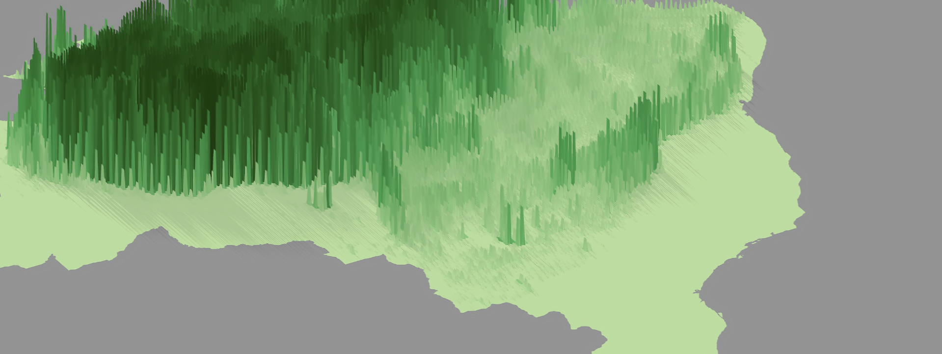
render_snapshot("brazil_forest_height_2019.png", clear=T)Aaaaand, here is the map! 🤩 It looks different from the original post because we used a more recent data for our tutorial.

Alright, that’s all ladies and gents! In this tutorial, you learned how to load and analyze huge raster files and create a 3D map based on the computed values. And all this was done in R! Feel free to check the full code here, clone the repo and reproduce, reuse and modify the code as you see fit.
This tutorial opens the doors for you to map tree height for other countries using the GLAD dataset. In fact, you can tweak my code a bit and make a 3D tree height map of any country in the world. On the bottom of this page you will find the links to raster files for other (sub)continents. Just plug any of them into url in 2. LOAD FOREST RASTER and run the code. Try it out and let me know how it goes!
I’d be happy to hear your view on how this map could be improved or extended to other geographic realms. To do so, please follow me on Twitter, Instagram or Facebook! Also, feel free to support my work by buying me a coffee here!