
How to overlay spatial polygons on satellite imagery using R
June 06, 2021 | Milos Popovic
Last Saturday we observed the World Environment Day under a slogan “Reimagine.Recreate.Restore.” As our world loses a forest the size of an average football stadium every 3 seconds, this slogan becomes a plea to do our best to help heal the nature. The United Nations has launched the UN Decade on Ecosystem Restoration (2021-2030) aimed at breathing new life into forests and farmlands across the globe. Forests cover nearly a third of our planet’s surface and turn carbon dioxide into oxygen. In the last two decades, deforestation has rapidly spread across Europe 😔. Recent study finds that Europe’s deforestation area has increased by almost 50% in 2015–2018 compared to 2011–2015.
In this post, we’ll explore the current state of forest cover in Europe. We’ll learn how to overlay commune spatial polygons over forest cover satellite imagery to compute and map the average percentage of the land area under forest using no more than 200 lines of code in R. Even better, you’ll be able to employ insights from this tutorial to overlay other spatial datasets (e.g. city districts, provinces, regions and countries) over any satellite data, from temperatures and active fires to land cover and pollution. Wow 😮!
In this tutorial, we’ll use the forest cover data from the one and only Global Land Cover data managed by Copernicus Monitoring Services. We’ll also download the shapefile of over 122,000 communes in Europe from Eurostat’s GISCO repo and overlay this shapefile on the forest cover data. Then we’ll use library exactextractr to compute the average value of each forest cover cell that intersects the community polygons, weighted by the percent of the cell that is covered. This will yield the average percentage of the forest cover for a specific community.
We’ll kick off this tutorial by loading the necessary libraries such as dplyr for data processing; sf for importing our communes shapefile; and raster for loading satellite imagery in .tif format. Also, we’ll load gdalUtils to be able to merge multiple rasters into a single file as well as the aforementioned exactextractr for computing weighted forest cover averages. Finally, we’ll call ggplot2 for mapping and package classInt will come in handy for constructing a discrete legend.
# install libraries
if(!require("dplyr")) install.packages("dplyr")
if(!require("sf")) install.packages("sf")
if(!require("raster")) install.packages("raster")
if(!require("gdalUtils")) install.packages("gdalUtils")
if(!require("exactextractr")) install.packages("exactextractr")
if(!require("ggplot2")) install.packages("ggplot2")
if(!require("classInt")) install.packages("classInt")

# load libraries
library(dplyr, quietly=T) # data processing
library(sf, quietly=T) # import polygons
library(raster, quietly=T) #load rasters
library(gdalUtils, quietly=T) # merge rasters
library(exactextractr, quietly=T) # zonal statistics
library(ggplot2, quietly=T) # map
library(classInt, quietly=T) # legend
We’ll first download the fractional forest cover data from the Copernicus Global Cover Land repo for the most recent year (2019). Btw, the fraction of forest cover corresponds to the fraction of ground covered by trees. This means that our satellite imagery data includes the percentage of land area under forest for every cell. We’ll use this info to calculate average percentage values for every commune in a bit.
The forest cover dataset is available as either a single raster file (>5 GB) or a series of raster files (1.1 GB for Europe) We’ll download and merge the 13 raster files for the territory of Europe to minimize our downloading time. Once we define all 13 URLs, we run a loop that starts downloading the files to our working directory.
# define the 2019 urls
urls <- c(
"https://s3-eu-west-1.amazonaws.com/vito.landcover.global/v3.0.1/2019/E000N80/E000N80_PROBAV_LC100_global_v3.0.1_2019-nrt_Tree-CoverFraction-layer_EPSG-4326.tif",
"https://s3-eu-west-1.amazonaws.com/vito.landcover.global/v3.0.1/2019/W040N80/W040N80_PROBAV_LC100_global_v3.0.1_2019-nrt_Tree-CoverFraction-layer_EPSG-4326.tif",
"https://s3-eu-west-1.amazonaws.com/vito.landcover.global/v3.0.1/2019/W020N80/W020N80_PROBAV_LC100_global_v3.0.1_2019-nrt_Tree-CoverFraction-layer_EPSG-4326.tif",
"https://s3-eu-west-1.amazonaws.com/vito.landcover.global/v3.0.1/2019/E020N80/E020N80_PROBAV_LC100_global_v3.0.1_2019-nrt_Tree-CoverFraction-layer_EPSG-4326.tif",
"https://s3-eu-west-1.amazonaws.com/vito.landcover.global/v3.0.1/2019/E040N80/E040N80_PROBAV_LC100_global_v3.0.1_2019-nrt_Tree-CoverFraction-layer_EPSG-4326.tif",
"https://s3-eu-west-1.amazonaws.com/vito.landcover.global/v3.0.1/2019/E040N60/E040N60_PROBAV_LC100_global_v3.0.1_2019-nrt_Tree-CoverFraction-layer_EPSG-4326.tif",
"https://s3-eu-west-1.amazonaws.com/vito.landcover.global/v3.0.1/2019/W020N60/W020N60_PROBAV_LC100_global_v3.0.1_2019-nrt_Tree-CoverFraction-layer_EPSG-4326.tif",
"https://s3-eu-west-1.amazonaws.com/vito.landcover.global/v3.0.1/2019/E000N60/E000N60_PROBAV_LC100_global_v3.0.1_2019-nrt_Tree-CoverFraction-layer_EPSG-4326.tif",
"https://s3-eu-west-1.amazonaws.com/vito.landcover.global/v3.0.1/2019/E020N60/E020N60_PROBAV_LC100_global_v3.0.1_2019-nrt_Tree-CoverFraction-layer_EPSG-4326.tif",
"https://s3-eu-west-1.amazonaws.com/vito.landcover.global/v3.0.1/2019/W020N40/W020N40_PROBAV_LC100_global_v3.0.1_2019-nrt_Tree-CoverFraction-layer_EPSG-4326.tif",
"https://s3-eu-west-1.amazonaws.com/vito.landcover.global/v3.0.1/2019/E000N40/E000N40_PROBAV_LC100_global_v3.0.1_2019-nrt_Tree-CoverFraction-layer_EPSG-4326.tif",
"https://s3-eu-west-1.amazonaws.com/vito.landcover.global/v3.0.1/2019/E020N40/E020N40_PROBAV_LC100_global_v3.0.1_2019-nrt_Tree-CoverFraction-layer_EPSG-4326.tif",
"https://s3-eu-west-1.amazonaws.com/vito.landcover.global/v3.0.1/2019/E040N40/E040N40_PROBAV_LC100_global_v3.0.1_2019-nrt_Tree-CoverFraction-layer_EPSG-4326.tif"
)

#DOWNLOAD FILES
for (url in urls) {
    download.file(url, destfile = basename(url), mode="wb")
}
In order to import raster files, we first enlist them using list.files. Since we want to import these rasters as a single file we use mosaic_rasters to declare the composition and name of the aggregated file (2019_forest_cover.tif). With the help of the stack function we merge our raster files and reproject ras to WGS84.
# enlist raster files, merge them into a single file and re-project
rastfiles <- list.files(path = getwd(),
pattern = ".tif$",
all.files=T,
full.names=F)
r <- mosaic_rasters(gdalfile=rastfiles,
dst_dataset="2019\_forest\_cover.tif",
of="GTiff")
raster <- '2019\_forest\_cover.tif'
ras <- stack(raster)
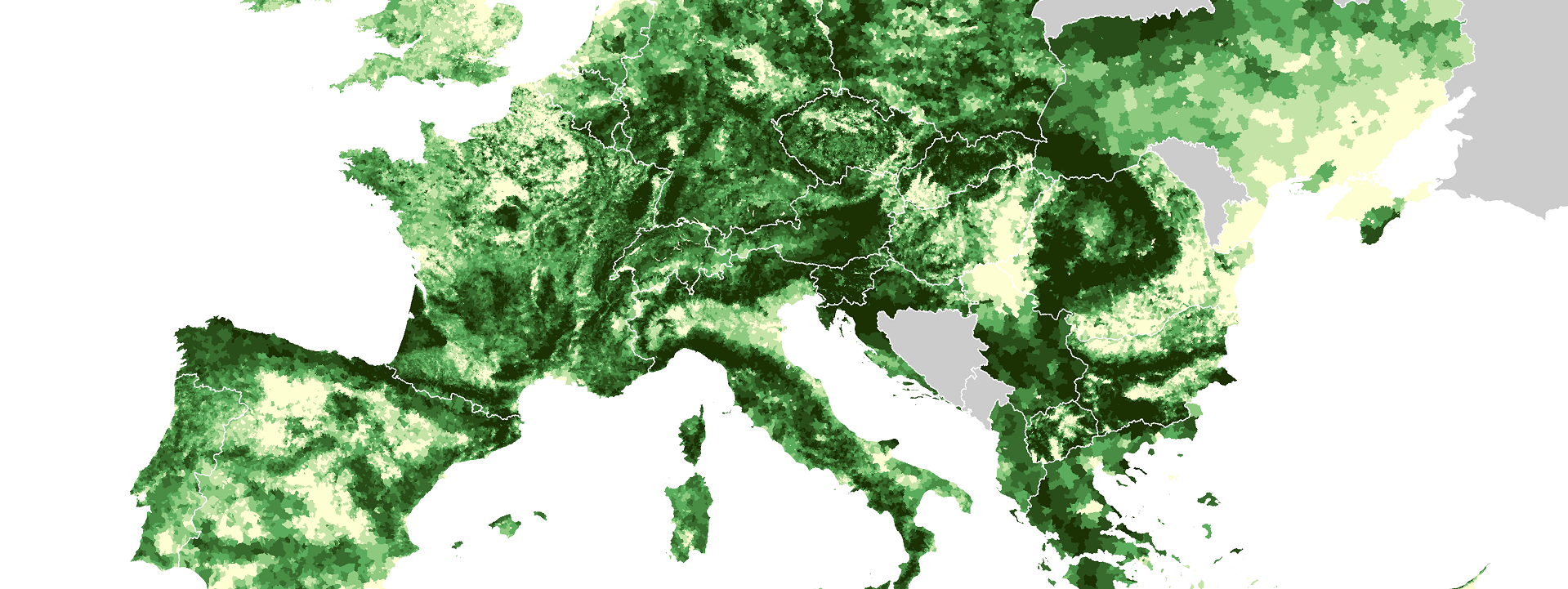
crs(ras) <- "+proj=longlat +datum=WGS84 +no_defs +ellps=WGS84 +towgs84=0,0,0"You should be able to see the image below after printing the object via plot(ras).

For our tutorial, we’ll use the micro-level spatial data on communes, which are human settlements at the lowest geographic level. We define the source URL and download the commune vector map. We then repeat the process and download the country-level shapefile. Using st_read we import our communes (and get rid of Greenland) and store the file into the com object; we also load the country-level data and store the file into the states object.
Alternatively, you could use library giscoR and download each of these shapefiles suing a fewer lines of code if you have R version 3.6.0 or newer. Because I work on version 3.5.1 we’ll stick to the vanilla approach 😋.
#DOWNLOAD SHAPEFILES
#Communities 2016 shapefile
url <- "https://gisco-services.ec.europa.eu/distribution/v2/communes/download/ref-communes-2016-01m.shp.zip"
download.file(url, basename(url), mode="wb")
unzip("ref-communes-2016-01m.shp.zip")
unzip("COMM_RG_01M_2016_4326.shp.zip")

#Eurostat 2013 country shapefile
url <- "https://gisco-services.ec.europa.eu/distribution/v2/countries/download/ref-countries-2013-01m.shp.zip" # location on the Eurostat website
download.file(url, basename(url), mode="wb") #download Eurostat country shapefiles
unzip("ref-countries-2013-01m.shp.zip") # unzip the boundary data
unzip("CNTR_RG_01M_2013_4326.shp.zip")

#load shapefiles
#communities
com <- st_read("COMM_RG_01M_2016_4326.shp",
			  stringsAsFactors = FALSE) %>%
  	   st_transform(4326) %>%
       st_as_sf() %>%
       dplyr::filter(!CNTR_ID%in%"GL") #remove Greenland

#countries
states <- st_read("CNTR_RG_01M_2013_4326.shp",
			  stringsAsFactors = FALSE) %>%
  	   st_transform(4326) %>%
       st_as_sf()
Sadly, the commune shapefile lacks info on Belarus, Bosnia-Herzegovina, Montenegro, Moldova and Russia. In our map of Europe, we’ll feature these countries as missing and remove non-European countries. In object cn1 we filter out these 5 countries including the neighboring countries in the Middle East and North Africa. The resulting data will serve as the basis for plotting national borders of the remaining countries. We also create another object cn2, which we’ll subsequently use to fill in the missing national polygons.
#only European countries (except those below) for border lines
out <- c("MA", "TN", "DZ", "EG",
		 "LY", "JO", "IL", "PS",
		 "SY", "SA", "LB", "IQ",
		 "IR", "GL", "BY", "BA",
		 "ME", "MD", "RU")
cn1 <- subset(states, !FID%in%out)

# extract Belarus, Bosnia-Herzegovina, Moldova, Montenegro and Russia
ins <- c("BY", "BA", "ME", "MD", "RU")
cn2 <- subset(states, FID%in%ins)
We are all set for our geospatial analysis! Using exact_extract we declare ras as our raster object; com as our spatial polygon object; and “mean” as the function to compute weighted averages of forest cover for every commune. The function returns object df, which is a vector of average fraction cover (in %) for every commune in the order of apperance in com. This allows us to use cbind to merge the two objects. We also rename our averages column to “values”.
#ANALYSIS
df  <- exact_extract(ras, com, "mean")
f <- cbind(com, df) %>%
     st_as_sf()
names(f)[12] <- "values"
We will use a discrete scale to show the average weighted forest cover fraction as it offers a better overview of the colors in the plot. We’ll first calculate the natural interval of our measure using quantile breaks for 8 cutpoints.
#LEGEND
# let's find a natural interval with quantile breaks
ni = classIntervals(f$values,
	            n = 8,
	            style = 'quantile')$brks
Next we’ll make our labels based on the cutpoints and round them to get rid of the decimal places.
# this function uses above intervals to create categories
labels <- c()
for(i in 1:length(ni)){
    labels <- c(labels, paste0(round(ni[i], 0),
                             "–",
                             round(ni[i + 1], 0)))
}
labels <- labels[1:length(labels)-1]
Finally, we’ll make the categorical variable (cat) based on the cutpoints.
# finally, carve out the categorical variable
# based on the breaks and labels above
f$cat <- cut(f$values,
              breaks = ni,
              labels = labels,
              include.lowest = T)
levels(f$cat) # let's check how many levels it has (8)
You remember that we lack the data on 5 European countries. So, we have to create a new “No data” category, which will be eventually depicted in grey.
# label NAs, too
lvl <- levels(f$cat)
lvl[length(lvl) + 1] <- "No data"
f$cat <- factor(f$cat, levels = lvl)
f$cat[is.na(f$cat)] <- "No data"
levels(f$cat)
Before we dive into mapping we want our map to include only European countries in the Lambert projection. We, therefore, have to create a bounding box and reproject the coordinates to the Lambert projection. First, we define the WGS84 projection as crsLONGLAT and the Lambert projection as crsLAEA. Next, we run st_sfc to create a bounding box conveniently labeled bb with the latitude and longitude coordinates under the WGS84 definition. Finally, we transform bb into the Lambert projection using st_transform and make a bounding box b with reprojected coordinates by running st_bbox(laeabb)
# MAPPING
# define projections
crsLONGLAT <- "+proj=longlat +datum=WGS84 +no_defs"
crsLAEA <- "+proj=laea +lat_0=52 +lon_0=10 +x_0=4321000 +y_0=3210000 +datum=WGS84 +units=m +no_defs"
#create a bounding box
bb <- st_sfc(
  st_polygon(list(cbind(
    c(-10.6600, 35.00, 35.00, -10.6600, -10.6600), # x-coordinates (longitudes) of points A,B,C,D
    c(32.5000, 32.5000, 71.0500, 71.0500, 32.5000)     # y-coordinates (latitudes) of points A,B,C,D
    ))),
  crs = crsLONGLAT)
# tranform to Lambert projection
laeabb <- st_transform(bb, crs = crsLAEA)
b <- st_bbox(laeabb) #create a bounding box with new projection
At last, we are ready to plot our map of forest cover in Europe. We will use 4 objects to create our map. Let’s recap:
- f is the main object with info on forest cover percentages;
- cn1 is the country-level spatial object with all the countries except the 5 missing European countries and Europe’s neighboring countries;
- cn2 is the country-level spatial object with 5 missing European countries;
- b denotes the bounding box in the Lambert projection.
We first plot the average forest cover using geom_sf argument with discrete cutpoints from our cat feature. Note that I’ll omit commune borders via color=NA to avoid intensive computation and messy map. But we’ll add national boundaries using geom_sf(data=cn1, fill=“transparent”, color=“white”, size=0.2). Note that this line will add national borders for all the European countries except those 5 missing. In the following chunk, we’ll fill the missing country polygons and lines using geom_sf(data=cn2, fill=“grey80”, color=“white”, size=0.2).
Since we aim to narrow our view to Europe, we run coord_sf; set our latitude and longitude limits based on the bounding box through xlim = c(b[“xmin”], b[“xmax”]), ylim = c(b[“ymin”], b[“ymax”]); and choose the Lambert projection via crs = crsLAEA.
Once again, we’ll paint our choropleth map using a manual color palette from Adobe Color and make it colorblind friendly with the help of Chroma.js Color Palette Helper. We’ll also modify the last numeric label to indicate that it encompasses all the values higher than 52.
map <-
ggplot() +
geom_sf(data=f, aes(fill=cat), color=NA) +
geom_sf(data=cn1, fill="transparent", color="white", size=0.2) + #lines
geom_sf(data=cn2, fill="grey80", color="white", size=0.2) + #missing Euro countries
coord_sf(crs = crsLAEA, xlim = c(b["xmin"], b["xmax"]), ylim = c(b["ymin"], b["ymax"])) +
labs(y="", subtitle="at community level",
         x = "",
         title="Fractional forest cover density in 2019",
         caption="©2021 Milos Popovic https://milospopovic.net\nSource: Buchhorn, M. et al. Copernicus Global Land Cover Layers — Collection 2.\nRemote Sensing 2020, 12, Volume 108, 1044. DOI 10.3390/rs12061044")+
scale_fill_manual(name= "average % forest cover",
  values=rev(c("grey80", '#1b3104', '#294d19', '#386c2e',
  			  '#498c44', '#5bad5d', '#8dc97f', '#c4e4a7',
  			  '#fefed3')),
  labels=c("0–6",     "6–10",    "10–15",   "15–21",   "21–29",   "29–39",   "39–52",
			">52",   "No data"),
  drop=F)+
guides(fill=guide_legend(
            direction = "horizontal",
            keyheight = unit(1.15, units = "mm"),
            keywidth = unit(15, units = "mm"),
            title.position = 'top',
            title.hjust = 0.5,
            label.hjust = .5,
            nrow =1,
            byrow = T,
            #labels = labs,
            # also the guide needs to be reversed
            reverse = F,
            label.position = "bottom"
          )
    ) +
theme_minimal() +
theme(text = element_text(family = "georg"),
panel.background = element_blank(),
legend.background = element_blank(),
legend.position = c(.45, .04),
panel.border = element_blank(),
panel.grid.minor = element_blank(),
panel.grid.major = element_line(color = "white", size = 0.2),
plot.title = element_text(size=22, color='#478c42', hjust=0.5, vjust=0),
plot.subtitle = element_text(size=18, color='#86cb7a', hjust=0.5, vjust=0),
plot.caption = element_text(size=9, color="grey60", hjust=0.5, vjust=10),
axis.title.x = element_text(size=10, color="grey20", hjust=0.5, vjust=-6),
legend.text = element_text(size=9, color="grey20"),
legend.title = element_text(size=10, color="grey20"),
strip.text = element_text(size=12),
plot.margin     =   unit(c(t=1, r=-2, b=-1, l=-2),"lines"), #added these narrower margins to enlarge maps
axis.title.y = element_blank(),
axis.ticks = element_blank(),
axis.text.x = element_blank(),
axis.text.y = element_blank())

Alright, this was all folks! In this tutorial, I showed you how to effortlessly download satellite imagery, calculate the average forest cover values for every polygon and create a beautiful map using R, ggplot2 and sf. This tutorial opens the gateway to overlaying spatial polygons over raster files. For example, you could analyze the size of urbanized areas in your country using this tutorial. Such projects could help you or your stakeholders better understand various environmental patterns on any geo level.
If you are wondering how you could easily apply this tutorial to similar data, here’s a hint: apart from the forest cover dataset, The Copernicus Global Land Cover data includes other datasets such as cropland, built-up areas or the snow and ice cover. If you wish to download any of these datasets for Europe, you could easily tweak my code as follows:
- copy the abovementioned URLs to forest cover raster files into your text editor;
- select all URLs and press Ctrl+H. This will open a window to find and replace a keyword;
- choose a keyword from the table below and replace the default Tree string with desired keyword.
Then simply re-run the code and download the data you want. Same goes for specific years!
| Data | Keyword |
|---|---|
| Bare/sparse vegetation | Bare |
| Built-up areas | BuiltUp |
| Cropland | Crops |
| Herbaceous vegetation | Grass |
| Moss and Lichen | MossLichen |
| Seasonal inland water | SeasonalWater |
| Shrubland | Shrub |
| Snow and Ice | Snow |
| Permanent inland water | PermanentWater |
Feel free to check the full code here, clone the repo and reproduce, reuse and modify the code as you see fit. As shown above, you’ll be able to produce a myriad of maps using the Copernicus satellite imagery programmatically in R with a slight modification of this code.
I’d be happy to hear your view on how this map could be improved or extended to other geographic realms. To do so, please follow me on Twitter, Instagram or Facebook!