
Mapping OSM and satellite data with terra in R
September 22, 2022 | Milos Popovic
More than a half of the world’s population lives in cities and the number is expected to rise to two-thirds by 2050! 😯 As our soil rapidly turns into asphalt and concrete, we often find ourselves as mere bystanders in the whole process.
But satellite technology helps us break the chains and witness the rise of cities first hand. In this tutorial, I will show you how to capture the expansion of built-up surfaces in the world’s largest urban areas. We will use the fascinating data on built-up change between 2000 and 2020 from the Global Land Analysis & Discovery (GLAD) data and OSM road data. Remember that we have already used their data on forest cover height to create a pretty 3D map of Brazil’s rainforest in this tutorial.
In the GLAD framework, built-up land is displayed as pixels that include examples of human-made surfaces such as roads, bridges, and buildings. The authors used a Convolutional Neural Network (CNN) algorithm for image recognition to assigns importance to input images and distinguish built-up from other land covers. Pretty cool, huh? Wait till you hear more: they further calibrated their data with building outlines and road data from the Open Street Map (OSM) to map the built-up areas for 2000 and 2020. This allows us to create highly-detailed maps of urban change paired with OSM roads for literally any place in the world. 😍
Let’s start our journey!
Load packages
In this tutorial, we call to arms several packages: tidyverse and sf for spatial analysis and data wrangling; terra for importing and working with raster files; osmdata for accessing OSM data in tidy format; and httr and XML for retrieving raster links from the GLAD website.
# libraries we need
libs <- c(
    "tidyverse", "sf",
    "osmdata", "terra",
    "httr", "XML", "lwgeom"
)

# install missing libraries
installed_libs <- libs %in% rownames(installed.packages())
if (any(installed_libs == F)) {
    install.packages(libs[!installed_libs])
}

# load libraries
invisible(lapply(libs, library, character.only = T))
Retrieve OSM data
Our priority is to define the city name (in our case that’s Delhi) and retrieve the bounding box so that we can crop the road and built-up data. Specifically, we use osmdata::getbb function to obtain city limits.
# 1. GET DELHI OSM DATA
#----------------------

city <- "Delhi, India"

get_bounding_box <- function() {
    bbox <- osmdata::getbb(city)
    return(bbox)
}

bbox <- get_bounding_box()
We print the bounding box and obtain the following latitude and longitude boundaries of Delhi. This piece of info will come in handy later in the tutorial.
bbox
       min      max
x 77.06194 77.38194
y 28.49172 28.81172
For now, let’s use the bounding box to clip the OSM road data. As you might remember from previous tutorials, OSM data recognizes multiple features. If you call osmdata::available_features() a list of over 100 available features unrolls in front of your eyes. Roads and links roads, along with special roads and paths are stored as “highway”. The complete list of 50 highway tags is visible upon executing available_tags(“highway”). Since we’d like to keep the map less polluted we limit our focus to roads and road links.
In the chunk below, we fetch OSM roads for the Delhi extent.
road_tags <- c(
    "motorway", "trunk",
    "primary", "secondary",
    "tertiary", "motorway_link",
    "trunk_link", "primary_link",
    "secondary_link", "tertiary_link"
)

get_osm_roads <- function() {

    roads <- bbox %>%
        opq() %>%
        add_osm_feature(
            key = "highway",
            value = road_tags
        ) %>%
        osmdata_sf()

    return(roads)
}

roads <- get_osm_roads()
Let’s have a look at Delhi’s major roads.
plot(sf::st_geometry(roads$osm_lines))

Download built-up change data
Our next step is to download the built-up change data for Delhi, which is stored in separate 10 x 10 degree extent files. In the following code, we scrap all the links from the website and place them into the list. While this step is not necessary when you fetch a single raster file, it’s useful for keeping the track of all available links in one place.
# 2. GET BUILT-UP DATA
#----------------------
# website
url <- "https://glad.umd.edu/users/Potapov/GLCLUC2020/Built-up_change_2000_2020/"

get_raster_links <- function() {
    # make http request
    res <- httr::GET(url)
    # parse data to html format
    parse <- XML::htmlParse(res)
    # scrape all the href tags
    links <- XML::xpathSApply(parse, path = "//a", xmlGetAttr, "href")
    # grab links only
    lnks <- links[-c(1:5)]
    # make all links and store in a list
    for (l in lnks) {
        rlinks <- paste0(url, lnks)
    }

    return(rlinks)
}

rlinks <- get_raster_links()
Once we retrieved all the possible links we go back to the bounding box to determine the file we need. This part requires a bit of guesswork. Since Delhi coordinates are around 30N for the longitude and 70E for the latitude, we would probably need the file that includes these degrees in the name. Let’s fetch it!
# bbox values
delhi_ext <- unname(c(
    bbox[1, ][1], bbox[1, ][2],
    bbox[2, ][1], bbox[2, ][2]
))

delhi_ext

77.06194 77.38194 28.49172 28.81172
Below we define the Delhi extent and grab the link. Then we download the extent from the link using terra::rast. The cool thing about this function is that the file is cached. In the following step, we crop the raster file to the Delhi extent, which will speed up our visualization down the road.
Raster file is a collection of pixels with values. We transform it into a data.frame with pixel values for every coordinate before passing it to ggplot2. Using terra::as.data.frame we get the data.frame with x, y and value columns. Finally, because the GLAD built-up dataset has three unique values (0 = no built-up area, 1 = built-up expansion 2000-2020, 2 = stable built-up area), we reshape the continuous into a categorical variable.
# create Delhi extent
de <- c(77.06194, 77.38194, 28.49172, 28.81172)

get_builtup_data <- function() {
    l <- rlinks[grepl("30N_070E", rlinks)]
    ras <- terra::rast(l)
    delhi_ras <- terra::crop(ras, de)
    df <- terra::as.data.frame(delhi_ras, xy = T)
    names(df)[3] <- "value"
    # define categorical values
    df$cat <- round(df$value, 0)
    df$cat <- factor(df$cat,
        labels = c("no built-up", "new", "existing")
    )

    return(df)
}

df <- get_builtup_data()
Visualization
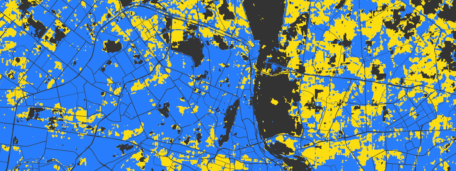
Let’s make the map, people! We have the Delhi data in place so our final task is to plot both the raster and roads data. We first apply the geom_raster function to data.frame derived from the raster file and choose cat to fill the polygons with our palette. Then we plot the roads data and choose the same color as the background to allow the built-up values to shine.
colrs <- c(
    "grey20", "#FCDD0F", "#287DFC"
)

p <- ggplot() +
    geom_raster(
        data = df,
        aes(x = x, y = y, fill = cat),
        alpha = 1
    ) +
    geom_sf(
        data = roads$osm_lines,
        color = "grey20",
        size = .1,
        alpha = 1,
        fill = "transparent"
    ) +
    scale_fill_manual(
        name = "",
        values = colrs,
        drop = F
    ) +
    guides(
        color = "none",
        fill = guide_legend(
            direction = "horizontal",
            keyheight = unit(1.5, units = "mm"),
            keywidth = unit(35, units = "mm"),
            title.position = "top",
            title.hjust = .5,
            label.hjust = .5,
            nrow = 1,
            byrow = T,
            reverse = F,
            label.position = "bottom"
        )
    ) +
    theme_minimal() +
    theme(
        axis.line = element_blank(),
        axis.text.x = element_blank(),
        axis.text.y = element_blank(),
        axis.ticks = element_blank(),
        axis.title.x = element_blank(),
        axis.title.y = element_blank(),
        legend.position = c(.5, .9),
        legend.text = element_text(size = 60, color = "white"),
        legend.title = element_text(size = 80, color = "white"),
        legend.spacing.y = unit(0.25, "cm"),
        panel.grid.major = element_line(color = "grey20", size = 0.2),
        panel.grid.minor = element_blank(),
        plot.title = element_text(
            size = 80, color = "grey80", hjust = .5, vjust = -30
        ),
        plot.caption = element_text(
            size = 40, color = "grey90", hjust = .5, vjust = 65
        ),
        plot.subtitle = element_text(
            size = 22, color = "#f5de7a", hjust = .5
        ),
        plot.margin = unit(
            c(t = -5, r = -4.5, b = -4.5, l = -5), "lines"
        ),
        plot.background = element_rect(fill = "grey20", color = NA),
        panel.background = element_rect(fill = "grey20", color = NA),
        legend.background = element_rect(fill = "grey20", color = NA),
        legend.key = element_rect(colour = "white"),
        panel.border = element_blank()
    ) +
    labs(
        x = "",
        y = NULL,
        title = "Built-up Land Change in Delhi, 2000-2020",
        subtitle = "",
        caption = "©2022 Milos Popovic (https://milospopovic.net) | Data: ©2022 Milos Popovic (https://milospopovic.net) | Data: GLAD Buil-up Change Data & ©OpenStreetMap contributors"
    )

ggsave(
    filename = "delhi_built_up.png",
    width = 6, height = 9, dpi = 600,
    device = "png", p
)
Hurray, here is the final map! 😍

And, that’s all, folks! In this tutorial, you learned how to map built-up expansion of Delhi using the satellite and OSM data in less than 200 lines of code and all that in R! Feel free to check the full code here, clone the repo and reproduce, reuse and modify the code as you see fit.
I’d be happy to hear your view on how this map could be improved or extended to other geographic realms. To do so, please follow me on Twitter, Instagram or Facebook! Also, feel free to support my work by buying me a coffee here!