Satellite images of Earth at night are some of the most breathtaking pictures of our beloved planet. With fascinating sceneries of the lit-up cities, night lights have been a source of inspiration for artists, businesspeople, reserchers and laypersons.

I, too, couldn’t resist the temptation of making nightlights map. At the beginning of this year, I wrote a tutorial on how to create a timelapse map of nightlights in Europe over the past 30 years. But I stopped short of mapping other continets or perspectives. So, in this tutorial I’d like to revisit this topic from a different angle and show you how to display your satellite data on a globe. Wow 😍!

A few years back, NASA scientists removed the moonlight, fires, and other natural sources of light to create the clearest image of Earth at night. In this tutorial, we will use NASA’s Black Marble data to display the shiny lights on the globe. You will learn how to apply an orthographic projection to make a pretty map of Earth at night.

Let’s begin!

Import libraries

As usual, we import a few libraries: tidyverse and sf for spatial analysis and data wrangling; giscoR for importing the world shapefile; terra for manipulating raster data; terrainr for plotting a multi-band raster; and magick for map annotation.

# libraries we need
libs <- c(
    "tidyverse", "sf", "giscoR",
    "mapview", "terra", "terrainr",
    "magick"
)

# install missing libraries
installed_libs <- libs %in% rownames(installed.packages())
if (any(installed_libs == F)) {
    install.packages(libs[!installed_libs])
}

# load libraries
invisible(lapply(libs, library, character.only = T))

World map polygon

First, we define two projections. One of them is the standard longitude/latitude projection, and the other is the Azimuthal orthographic projection. We use the former to project our map to WGS84 and then apply the latter to turn the flat Earth into a globe.

# define projections
longlat_crs <- "+proj=longlat +datum=WGS84 +no_defs"
ortho_crs <-'+proj=ortho +lat_0=32.4279 +lon_0=53.688 +x_0=0 +y_0=0 +R=6371000 +units=m +no_defs +type=crs'

In the next step, we retrieve the world polygon. We will use this polygon to crop the nightlight data.

get_flat_world_sf <- function() {
    world <- giscoR::gisco_get_countries(
        year = "2016",
        epsg = "4326",
        resolution = "10"
    ) %>%
        sf::st_transform(longlat_crs)

    world_vect <- terra::vect(world)

    return(world_vect)
}

world_vect <- get_flat_world_sf()

NASA’s nightlight data

We are now ready to download NASA’s data. Here we opt for the latest 2017 data in the lowest possible resolution 3600x1800 in order to make our life easier. Thanks to terra package, we can import the file directly into R. Next, we crop the raster file so that it fits the world map coordinates.

# 2. NASA DATA
#-------------
get_nasa_data <- function() {
    ras <- terra::rast("/vsicurl/https://eoimages.gsfc.nasa.gov/images/imagerecords/144000/144898/BlackMarble_2016_01deg_geo.tif")
    rascrop <- terra::crop(x = ras, y = world_vect, snap = "in")
    ras_latlong <- terra::project(rascrop, longlat_crs)
    ras_ortho <- terra::project(ras_latlong, ortho_crs)
    return(ras_ortho)
}

ras_ortho <- get_nasa_data()

Next, we project the satellite imagery into the longlat projection and retrieve a flat world map of nightlights below.

Finally, we project the raster file once more and retrieve the globe map.

Hmmmm, hold on, there seems to be a white circle over the North Pole 😒. This looks like missing data! We better fill those gaps by assigning the lowest value (black) to the blank spots.

r <- ifel(is.na(ras_ortho), 0, ras_ortho)
plot(r)

Much better! 😊

Mapping nightlight data

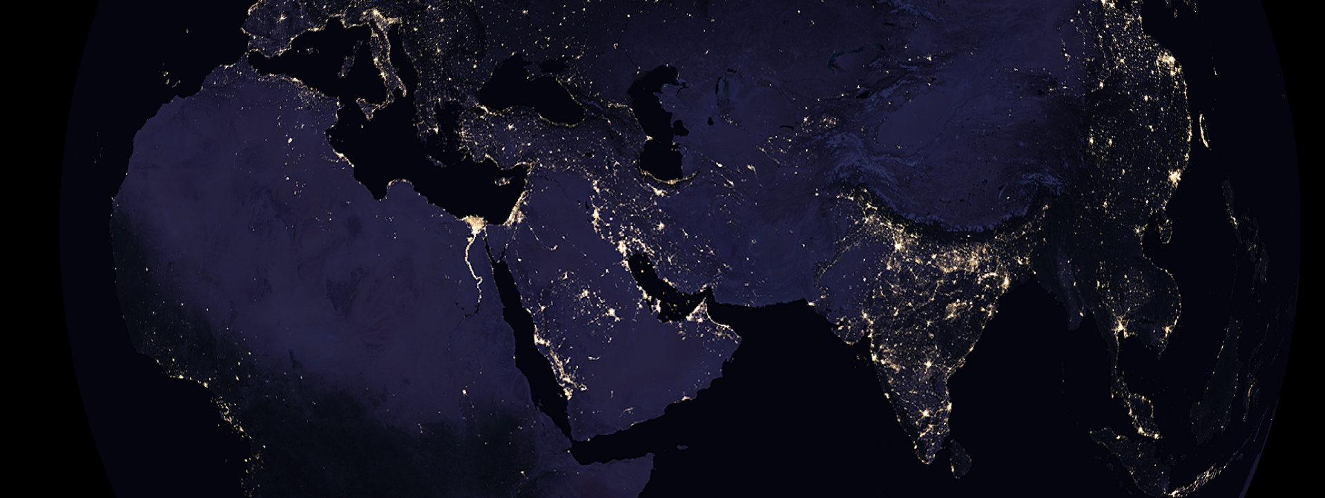
It’s time to make the map, people! In the chunk below, we will create and run a function that creates a globe centered on a the midpoint of Africa, Asia and Europe.

Our raster is a multi-band raster, meaning that we have three color layers for the same spatial area. We could transform our raster data into a data.frame before plotting it in ggplot2. But this is computer-intensive and tends to throw the no memory error. Instead, we use geom_spatial_rgb function from terrainr. This function allows us to plot a three-band RGB raster in ggplot2, using these layers as background base maps for other spatial plotting while keeping the raster format. Finally, we’ll use black as a background for our plot in order to match the darkest color value on our globe.

# 3. MAP NIGHTLIGHTS
#-------------------
make_nighlights_globe <- function() {
    globe <- ggplot() +
        terrainr::geom_spatial_rgb(
            data = r,
            mapping = aes(
                x = x,
                y = y,
                r = red,
                g = green,
                b = blue
            )
        ) +
        theme_minimal() +
        theme(
            plot.margin = unit(
                c(t = -1, r = -1, b = -1, l = -1), "lines"
            ),
            panel.grid.major = element_blank(),
            panel.grid.minor = element_blank(),
            plot.background = element_rect(fill = "black", color = NA),
            panel.background = element_rect(fill = "black", color = NA),
            legend.background = element_rect(fill = "black", color = NA),
            panel.border = element_rect(fill = NA, color = "black"),
        ) +
        labs(
            x = "",
            y = "",
            title = "",
            subtitle = "",
            caption = ""
        )
}

globe <- make_nighlights_globe()

ggsave(
    filename = "nightlight_globe.png",
    width = 7, height = 7.5, dpi = 600, device = "png", globe
)

And this is the map! 😎

Using magick package to annotate our new map we place a cherry on top.

# 4. ANNOTATE MAP
#----------------
# read image
map <- magick::image_read("nightlight_globe.png")

# set font color
clr <- "#FFFFBC"

# Title
map_title <- magick::image_annotate(map, "Earth at night",
    font = "Georgia",
    color = alpha(clr, .65), size = 200, gravity = "north",
    location = "+0+80"
)

# Caption
map_final <- magick::image_annotate(map_title, glue::glue(
   "©2022 Milos Popovic (https://milospopovic.net) | ",
    "Data: NASA Earth Observatory"
),
font = "Georgia", location = "+0+50",
color = alpha(clr, .45), size = 50, gravity = "south"
)

magick::image_write(map_final, glue::glue("nightlight_globe_annotated.png"))

Alright, that’s all, folks! In this tutorial, you learned how to download, reproject and visualize NASA’s nightlight data in the form of world globe and all that in R! But this is not all: the elegance of this tutorial is that you can choose any midpoint for your map. You just need to pass coordinates to +lat_0 and +lon_0. For example, if you’d like to center your globe on the New York City like I did in the upper left corner of the image below you should define ortho_crs as follows:

ortho_crs <- "+proj=ortho +lon_0=-74.26 +lat_0=40.7 +x_0=0 +y_0=0 +R=6371000 +units=m +no_defs +type=crs" # New York

and re-run the script.

If you would like to replicate the remaining views from the image please copy and plug each of the following lines into your ortho_crs object, and re-run the script:

ortho_crs <- "+proj=ortho +lon_0=130.8 +lat_0=-12.4 +x_0=0 +y_0=0 +R=6371000 +units=m +no_defs +type=crs" #Darwin, Australia

ortho_crs <- "+proj=ortho +lon_0=-38.66 +lat_0=-3.8 +x_0=0 +y_0=0 +R=6371000 +units=m +no_defs +type=crs" #Fortaleza, Brazil

ortho_crs <- "+proj=ortho +lon_0=0 +lat_0=45 +x_0=0 +y_0=0 +R=6371000 +units=m +no_defs +type=crs" #North Pole

Feel free to check the full code here, clone the repo and reproduce, reuse and modify the code as you see fit.

I’d be happy to hear your view on how this map could be improved or extended to other geographic realms. To do so, please follow me on Twitter, Instagram or Facebook! Also, feel free to support my work by buying me a coffee here!