Motorway map of Europe using OSM data in R

Have you ever wondered how to create your own road map? Look no further: in this tutorial, I’ll show you how to make a motorway map of Europe 🤗! We’ll download the massive shapefile from OpenStreetMap (OSM) and import it into R. OSM is an editable, free, and open geo database of the world where a myriad of users around the globe continuously add geo location info and attributes such as amenities, roads, or rails to the server. Since OSM data are free of charge, anyone can download any data extract from this database on the continent, country or regional level. The zipped file includes geo point locations of interests (e.g. bars, gas stations and other amenities) and spatial lines (e.g. rivers, roads, railways). You can simply visit one of the OSM websites such as Geofabrik and download data from its server. And that’s exactly what we are going to do in this tutorial.

Let’s get to it! We will load only 2 packages this time:
sf for importing the motorway shapefile; and tidyverse for data wrangling and visualization. I’m a big fan of the Georgia font so we’ll use it for the title and labels in our map.

if(!require("sf")) install.packages("sf")
if(!require("tidyverse")) install.packages("tidyverse")  

library(tidyverse, quietly=T)
library(sf, quietly=T)

windowsFonts(georg = windowsFont('Georgia'))

We’ll first download the 24.4 GB Europe file with all the locations and attributes for the old continent. Sadly, that will consume a lot of your disk space 😬! Also, it’ll take some time to download the files depending on your Internet speed. However, I’m unaware of a more efficient approach to making such a detailed map. Another equally cumbersome and a bit slower approach is to use oe_get from the osmextract library.

Once we’ve downloaded the OSM Europe shapefile, we’ll need only motorways and motorway links for our project. So let’s write a SQL query to select only those features from the OSM file. Finally, we just got to import the Europe shapefile and transform it into WGS84 projection.

#download file
u <- "https://download.geofabrik.de/europe-latest.osm.pbf"
download.file(u, basename(u), mode="wb")

#query motorways
q = "SELECT highway 
    FROM lines 
    WHERE highway IN('motorway', 'motorway_link')"

mway <- st_read("europe-latest.osm.pbf", query = q)  %>% 
        st_transform(4326) %>% 
        st_as_sf()

Next, we’ll download and unzip the Eurostat 2013 world shapefile.

url <- "https://gisco-services.ec.europa.eu/distribution/v2/countries/download/ref-countries-2013-01m.shp.zip"
download.file(url, basename(url), mode="wb")
unzip("ref-countries-2013-01m.shp.zip")
unzip("CNTR_RG_01M_2013_4326.shp.zip")

We only need European countries but the Eurostat shapefile has no info on continents. Luckily, there is a column on ISO2 country codes so we just need to download a list of European countries with ISO2 codes and filter the shapefile. Because OSM data includes Turkey and Cyprus we also consider the ISO2 codes of these two countries.

urlfile <-'https://raw.githubusercontent.com/lukes/ISO-3166-Countries-with-Regional-Codes/master/all/all.csv'
iso2 <- read.csv(urlfile) %>%
        filter(region=="Europe" | alpha.2 == "TR" | alpha.2 == "CY") %>%
        select("alpha.2")

In the following chunk, we open the Eurostat world shapefile, correct the ISO2 country codes for Greece and the United Kingdom (for some reason, these were incorrect) and filter European countries plus Cyprus and Turkey. Now we have a national map of Europe as a basis for our motorway map!

europe <- read_sf("CNTR_RG_01M_2013_4326.shp",
            stringsAsFactors = F) %>%
         st_transform(4326) %>% 
         st_as_sf() %>%
         mutate(FID = recode(FID, 'UK'='GB')) %>% 
         mutate(FID = recode(FID, 'EL'='GR')) %>%
         subset(FID%in%iso2$alpha.2)

Just a few more steps before we venture into map-making. We’ll be using the Lambert projection so we first define this projection. Next we create a bounding box with WGS84 coordinates and transform these coordinates into the Lambert projection.

crsLONGLAT <- "+proj=longlat +datum=WGS84 +no_defs"
crsLAEA <- "+proj=laea +lat_0=52 +lon_0=10 +x_0=4321000 +y_0=3210000 +datum=WGS84 +units=m +no_defs"

bb <- st_sfc(
  st_polygon(list(cbind(
    c(-10.6600, 36.5500, 36.5500, -10.6600, -10.6600),
    c(34.5000, 34.5000, 71.0500, 71.0500, 34.5000)     
    ))),
  crs = crsLONGLAT)

laeabb <- st_transform(bb, crs = crsLAEA)
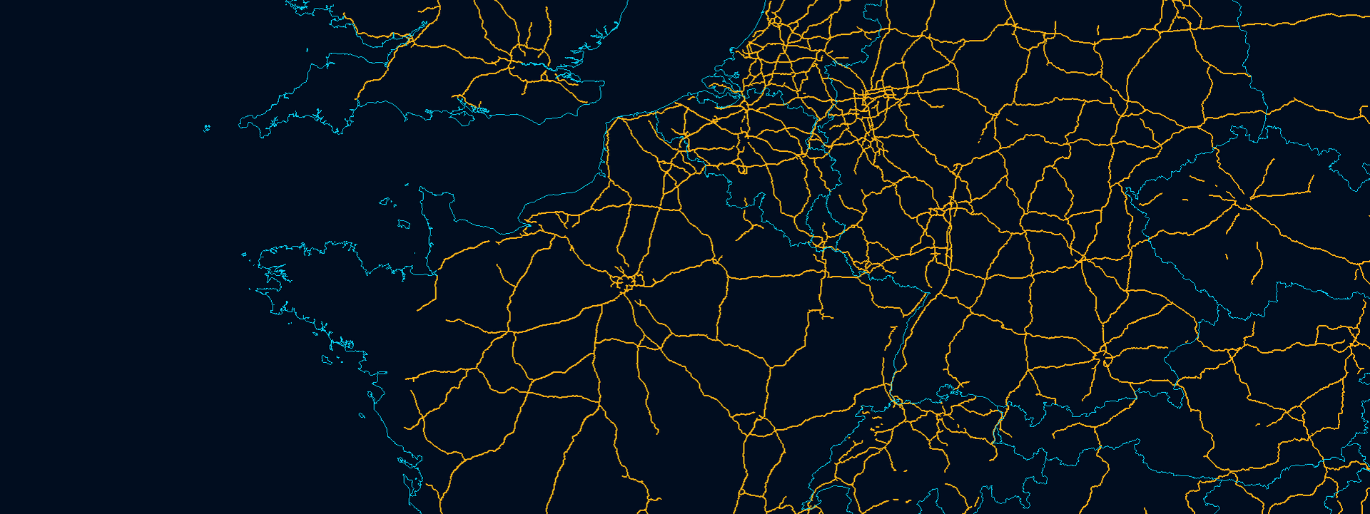
b <- st_bbox(laeabb)

Alright, ladies and gents, we’re ready to plot our motorway map of Europe. We first plot the motorway lines followed by the national map of Europe using geom_sf. The motorway lines are thicker than national boundaries but you can play with size and adjust the values.

Since we aim to narrow our view to Europe, we run coord_sf; set our latitude and longitude limits based on the bounding box through xlim = c(b[“xmin”], b[“xmax”]), ylim = c(b[“ymin”], b[“ymax”]); and choose the Lambert projection via crs = crsLAEA.

p <- ggplot() +
geom_sf(data=mway, color="#FFB115", size=0.15, fill=NA) +
geom_sf(data=europe, color="#07CFF7", size=0.1, fill=NA) +
    coord_sf(crs = crsLAEA, 
             xlim = c(b["xmin"], b["xmax"]), 
             ylim = c(b["ymin"], b["ymax"])) +
    theme_minimal() +
  theme(text = element_text(family = "georg", color = "#22211d"),
    axis.line = element_blank(),
    axis.text.x = element_blank(),
    axis.text.y = element_blank(),
    axis.ticks = element_blank(),
    axis.title.x = element_text(size=9, color="grey90", hjust=0.25, vjust=3),
    axis.title.y = element_blank(),
    legend.position = "none",
    legend.text = element_text(size=9, color="grey20"),
    legend.title = element_text(size=10, color="grey20"),
    panel.grid.major = element_line(color = "#010D1F", size = 0.2),
    panel.grid.minor = element_blank(),
    plot.title = element_text(face="bold", size=16, color="grey90", hjust=.5),
    plot.caption = element_text(size=8, color="grey90", hjust=1, vjust=0),
    plot.subtitle = element_text(size=12, color="grey20", hjust=.5),
    plot.margin = unit(c(t=1, r=-2, b=-1, l=-2),"lines"),
    plot.background = element_rect(fill = "#010D1F", color = NA), 
    panel.background = element_rect(fill = "#010D1F", color = NA), 
    legend.background = element_rect(fill = "#010D1F", color = NA),
    panel.border = element_blank()) +
    labs(x = "©2021 Milos Popovic (https://milospopovic.net)\n Data: © OpenStreetMap contributors", 
         y = NULL, 
         title = "European motorways", 
         subtitle = "", 
         caption = "")

ggsave(filename="eur_motorways.png", width= 7, height= 8.5, dpi = 600, device='png', p)

Aaaaand, voila! 🤩

Alright, that’s all folks! In this tutorial, you learned how to use big data to make a cool motorway map of Europe using fewer than 100 lines of code in R. This tutorial opens the doors for you to map your own motorway network for any continent. In fact, you can tweak my code a bit and make a motorway map of a specific country. Here is the list of all European countries available on the OSM GeoFabrik website.

Let’s take, for example, Austria. Replace the Europe URL with the URL for Austria where we download the motorway data. Then download the Eurostat world shapefile and filter Austria (ISO2 = AT). Finally, plot the motorway network in Austria.

Have a look at the full code here, clone the repo and reproduce, reuse and modify the code as you see fit. With a slight modification of this code, you’ll be able to produce a plethora of maps using the OSM big data programmatically in R.

I’d be happy to hear your view on how this map could be improved or extended to other geographic realms. To do so, please follow me on Twitter, Instagram or Facebook!