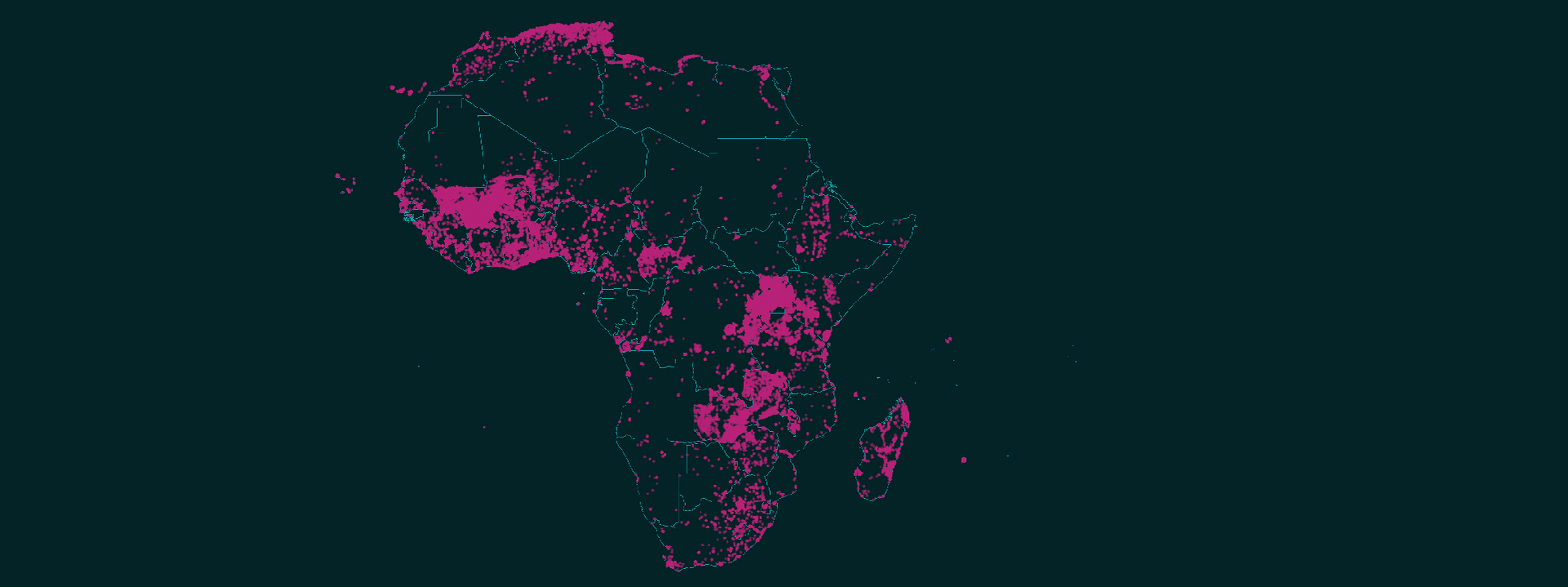
Map Africa using OSM data in R
November 04, 2022 | Milos Popovic
From roads to places of interest, OpenStreetMap (OSM) data is a springwell of free geospatial data. In my previous tutorials, we barely tapped into OSM’s gigantic reservoir to display motorways in Europe. One of the major problems that we encountered is that OSM data is huge. This means that mapping countries or continents is a painful process that requires downloading multiple files and gluing them together.
In this tutorial, you’ll learn how to download and extract OSM data for Africa in a simple and straightforward way. Wow 😍! And, that’s not all: my method will allow you to do the same for any other country or continent in the world!
Without further delay, let’s jump straight into the code!
Import packages
We need several essential libraries in this session. One set of libraries will help us scrape African country links from the OSM website. These include httr and XML. Another set of packages will help us process the data and includes tidyverse, sf and lwgeom for spatial analysis and data wrangling; and giscoR for importing the world shapefile.
# libraries we need
libs <- c(
    "tidyverse", "sf", "giscoR",
    "httr", "XML", "lwgeom", "stringr"
)

# install missing libraries
installed_libs <- libs %in% rownames(installed.packages())
if (any(installed_libs == F)) {
    install.packages(libs[!installed_libs])
}

# load libraries
invisible(lapply(libs, library, character.only = T))

# Montserrat font
# comment out these lines if you work on Linux or MacOS
sysfonts::font_add_google("Montserrat", "Montserrat")
showtext::showtext_auto()
Download OSM Africa data
Our first step is to download the Africa data from the Geofabrik website. You’ll notice that this page includes links to the country-level data. In the chunk below, we make a request, parse the data to the html format, scrape all the links from the website, and place them into a list. This returns a lot of garbage links so we use grepl to keep only links to the zipped shapefiles. Finally we remove .htmlafrica from our links.
# 1. DOWNLOAD AFRICA DATA
#------------------------

# Africa URL
url <- paste0("https://download.geofabrik.de/africa.html")
# download standard OSM country files
get_africa_links <- function() {
    # make http request
    res <- httr::GET(url)
    # parse data to html format
    parse <- XML::htmlParse(res)
    # scrape all the href tags
    links <- XML::xpathSApply(parse, path = "//a", XML::xmlGetAttr, "href")
    # grab links
    lnks <- links[-c(1:5)]
    # make all links and store in a list
    for (l in lnks) {
        all_links <- paste0(url, lnks)
    }

    africa_links <- all_links[grepl("latest-free.shp.zip", all_links)] %>%
        stringr::str_remove(".htmlafrica")

    return(africa_links)
}

africa_links <- get_africa_links()
If you run the function above, you should be able to see 55 links (see the truncated list below).
> africa_links
 [1] "https://download.geofabrik.de/africa/algeria-latest-free.shp.zip"
 [2] "https://download.geofabrik.de/africa/angola-latest-free.shp.zip"
 [3] "https://download.geofabrik.de/africa/benin-latest-free.shp.zip"
 [4] "https://download.geofabrik.de/africa/botswana-latest-free.shp.zip"
 [5] "https://download.geofabrik.de/africa/burkina-faso-latest-free.shp.zip"
We use a for loop to download all the files to the local drive.
# download files
for (a in africa_links) {
    download.file(a, destfile = basename(a), mode = "wb")
}
Pull together OSM Africa data
We downloaded 55 zipped files and we proceed to unzip them. Not so fast! Each zipped file holds several shapefiles for places of interest, roads, railroads, traffic, waterways etc. This is the full list of shapefiles available in a typical OSM zipped folder:
"gis_osm_buildings_a_free_1.shp"
"gis_osm_landuse_a_free_1.shp"
"gis_osm_natural_a_free_1.shp"
"gis_osm_natural_free_1.shp"
"gis_osm_places_a_free_1.shp"
"gis_osm_places_free_1.shp"
"gis_osm_pofw_a_free_1.shp"
"gis_osm_pofw_free_1.shp"
"gis_osm_pois_a_free_1.shp"
"gis_osm_pois_free_1.shp"
"gis_osm_railways_free_1.shp"
"gis_osm_roads_free_1.shp"
"gis_osm_traffic_a_free_1.shp"
"gis_osm_traffic_free_1.shp"
"gis_osm_transport_a_free_1.shp"
"gis_osm_transport_free_1.shp"
"gis_osm_water_a_free_1.shp"
"gis_osm_waterways_free_1.shp"
Now, every zipped folder that we downloaded from Geofabrik has the same contents and file names. So, R will overwrite every file that we use have unzipped until you are left with a single shapefile for the last unzipped country.
To avoid this scenario, we have to rename the shapefiles every time we unzip a file. Since every shapefile comes along with .cpg, .dbf, .prj, .shp, and .shx etensions we also have to make sure that we assign the identical name to each extension. Otherwise we won’t be able to open the shapefile.
So, we’ll first set our working directory. This is where the zipped files are stored. Then we list all the zipped files. Finally, we create a new folder where we’ll migrate the renamed unzipped files.
# 2. UNZIP AFRICAN PLACES
#------------------------

# unzipping and renaming
main_path <- getwd()

zip_files <- list.files(
    path = main_path,
    pattern = "*.zip", full.names = T
)

new_dir <- "unzipped_africa_osm"

dir.create(path = paste0("../", new_dir))

out_dir <- main_path %>%
    stringr::str_remove("africa") %>%
    paste0(new_dir)

setwd(out_dir) # setwd for rename/remove functions to work
In this tutorial, we will use only the places of interest (“pois”) shapefile. Instead of unzipping all the files we write a function that grabs only those files that contain “pois_free” in their name. Only in the next step do we unzip a pois file and place it into our newly created directory. In the next step, we create a sample number that we then append to the new file name. This way, we avoid overwriting unzipped files. 😎 Finally, we remove both the old and new file name vectors.
for (z in 1:length(zip_files)) {
    zip_names <- grep("pois_free", unzip(zip_files[z], list = T)$Name,
        ignore.case = T, value = T
    )

    unzip(zip_files[z], files = zip_names, exdir = out_dir, overwrite = F)
    x <- sample(1:length(zip_files), 1, replace = T)
    file_old <- c(list.files(out_dir)) # existing file names
    file_new <- c(paste0(x, "_", file_old))
    file.rename(
        paste0(out_dir, "/", file_old),
        paste0(out_dir, "/", file_new)
    )
    rm(file_old)
    rm(file_new) # Delete vectors from the environment
}
Extracting African schools
We have all the places of interest in store so let’s glue them together!
In this tutorial, we narrow our focus to primary and secondary schools in order to speed up the data wrangling and mapping. But if you check the fclass column in the OSM object you will find a long list of other amenities such as bakeries, banks, cafes, hospitals, restaurants etc.
We store all the files into a list and apply sf::st_read. This creates a list of sf objects. A simple do.call(rbind, pois_list) merges all the sf objects into a single sf object. In the final step, we filter African schools.
# 3. FILTER AFRICAN SCHOOLS
#--------------------------
get_africa_schools <- function() {
    pois_files <- list.files(
        path = out_dir,
        pattern = "*.shp", full.names = T
    )

    pois_list <- lapply(pois_files, sf::st_read)

    africa_pois <- do.call(rbind, pois_list)

    africa_schools <- africa_pois %>%
        dplyr::filter(fclass == "school")


    return(africa_schools)
}

africa_schools <- get_africa_schools()
Get Africa sf object
One last step before we map schools is to fetch the national map of Africa. As always, we call to arms giscoR.
# 4. MAP OF AFRICA
#-----------------
# load national map
get_africa_map <- function() {
    africa_map <- giscoR::gisco_get_countries(
        year = "2016",
        epsg = "4326",
        resolution = "3",
        region = "Africa"
    )

    return(africa_map)
}

africa_map <- get_africa_map()
Mapping African schools
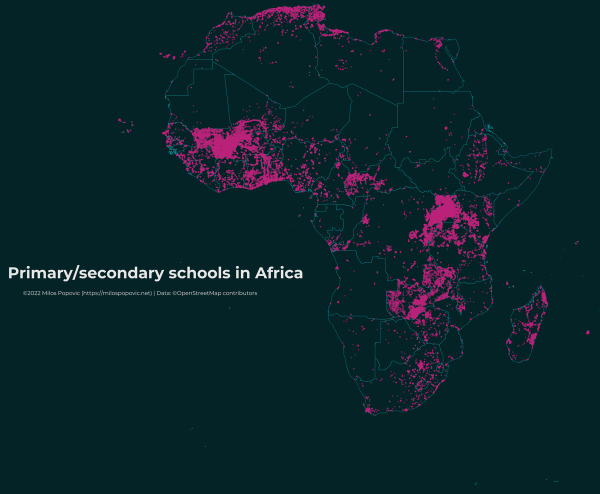
Alrighty, it’s time to make the map, folks!
In the chunk below, we will use pink points against a dark green background and light blue country lines. The African national map is transparent and the national borders are thin. For African schools, we also choose a small point size and low alpha value to make individual points stand out in the crowd. You can toy with these settings to create an even better map!
# 5. MAP
#-------
p <- ggplot() +
    geom_sf(
        data = africa_map,
        fill = "transparent", color = "#0FAAB8", size = .1
    ) +
    geom_sf(
        data = africa_schools,
        color = "#B82178", size = .05, fill = "#B82178",
        alpha = .45
    ) +
    theme_minimal() +
    theme(
        text = element_text(family = "Montserrat"), # remove this line if you work on Linux or MacOS
        axis.line = element_blank(),
        axis.text.x = element_blank(),
        axis.text.y = element_blank(),
        axis.ticks = element_blank(),
        axis.title.x = element_text(
            size = 35, color = "grey90", hjust = 0.25, vjust = 220
        ),
        axis.title.y = element_blank(),
        legend.position = "none",
        panel.grid.major = element_line(color = "#032326", size = 0),
        panel.grid.minor = element_blank(),
        plot.title = element_text(
            face = "bold", size = 100, color = "grey90", hjust = .25,
            vjust = -100
        ),
        plot.margin = unit(
            c(t = -10, r = -10, b = -10, l = -10), "lines"
        ),
        plot.background = element_rect(fill = "#032326", color = NA),
        panel.background = element_rect(fill = "#032326", color = NA),
        legend.background = element_rect(fill = "#032326", color = NA),
        panel.border = element_blank()
    ) +
    labs(
        x = "©2022 Milos Popovic (https://milospopovic.net) | Data: ©OpenStreetMap contributors",
        y = NULL,
        title = "Primary/secondary schools in Africa",
        subtitle = "",
        caption = ""
    )

ggsave(
    filename = "africa_schools.png",
    width = 8.5, height = 7, dpi = 600, device = "png", p
)
And here it is! 😎
That would be all, dear folks! In this tutorial, you learned how to bulk download, glue together and visualize OSM data and all that in R! But this is just a beginning of a beautiful friendship. You can use these insights to map other OSM features such as buildings, roads and waterways. Furthermore, you can use the data to calculate and visualize other important metrics such as road density or length. The use case for this tutorial extends far beyond Africa to encompass countries for which OSM data exists only on the sub-state level such as, for example, Canada, France, India, Indonesia, or Russia. I would be curious to know if you managed to pull off a similar analysis for these countries!
In the meantime, feel free to check the full code here, clone the repo and reproduce, reuse and modify the code as you see fit.
I’d be happy to hear your view on how this map could be improved or extended to other geographic realms. To do so, please follow me on Twitter, Instagram or Facebook! Also, feel free to support my work by buying me a coffee here!

