Make a railway map of Europe in R
May 21, 2022 | Milos Popovic
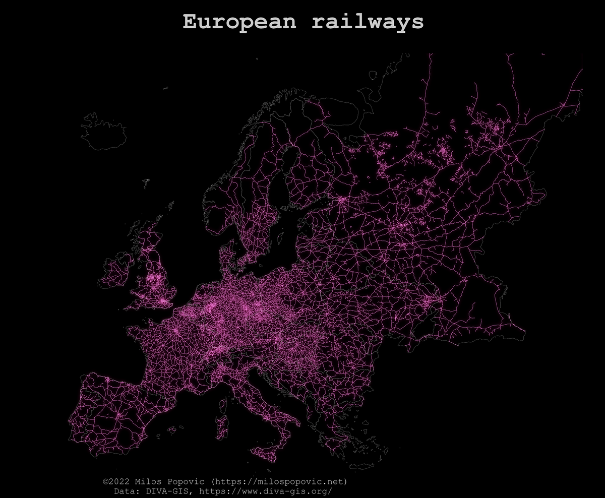
During my last week’s commute to work on a train I bumped into OpenRailwayMap, an OpenStreetMap (OSM)-based interactive map of railways 😍. Since I’m a fan of trains, I was thinking how we could bring this map to life using R. Previously I’ve manually downloaded and extracted rawilway lines from OSM to make the map below. But this was painful as I had to download the entire Europe file (25 GB) and process it in QGIS. It took hours!
My map shows European railways 🌍🚅🛤️#rail #railway #europe #osm #RStats #DataScience #dataviz #maps #rspatial pic.twitter.com/BUkuw3RfvA
— Milos Popovic (@milos_agathon) April 29, 2022
In this tutorial, we will take a shortcut to create a railway map of Europe programatically in R. For that matter, we will use DIVA-GIS, an app and open data source for mapping and geo analysis. Although DIVA-GIS was developed by a team of scholars to study the distribution of biodiversity the website has hidden GIS treasures such as national administrative units, rivers, roads, railways, all in in ESRI shapefile format.
Load libraries
Before we jump into data analysis, let’s import several libraries such as tidyverse and sf for data wrangling and geospatial analysis; giscoR for importing the shapefile of European countries; and ggfx to make our railways glow!
windowsFonts(georg = windowsFont('Georgia'))

# libraries we need
libs <- c("tidyverse", "sf", "giscoR", "ggfx")

# install missing libraries
installed_libs <- libs %in% rownames(installed.packages())
if (any(installed_libs == F)) {
  install.packages(libs[!installed_libs])
}

# load libraries
invisible(lapply(libs, library, character.only = T))
Bulk download railway shapefiles 📥
We will first bulk download the railway shapefiles for European countries. To do that, we fetch the list of European countries and select their respective ISO3 codes. We need those because the web links to railway shapefiles are annotated with ISO3 codes.
europeList <- function(urlfile, iso3DF) {

  urlfile <-'https://raw.githubusercontent.com/lukes/ISO-3166-Countries-with-Regional-Codes/master/all/all.csv'

  iso3DF <- read.csv(urlfile) %>%
        filter(region=="Europe") %>%
        select("alpha.3") %>%
        rename(iso3 = alpha.3)

  return(iso3DF)
}

iso3DF <- europeList()
If you inspect DIVA-GIS website you will notice that URLs for every country shapefile have the same root: https://biogeo.ucdavis.edu/data/diva/rrd/, followed by an ISO3 and .zip extension. So, we just need to iterate through the list of countries to create specific URLs. We create a temporary directory rail into which we’ll bulk download the shapefiles. Finally, we iterate through the list of URLs and download the zipped folders.
# create a directory for railway SHPs
dir <- file.path(tempdir(), 'rail')
dir.create(dir)

downloadSHP <- function(urls) {

        # make URL for every country
        urls <- paste0("https://biogeo.ucdavis.edu/data/diva/rrd/",
                iso3DF$iso3, "_rrd.zip")

        # iterate and download
        lapply(urls, function(url) download.file(url, file.path(dir, basename(url))))
}

downloadSHP()
Unzip and load the data 📁
Now we just need to unzip and load the shapefiles. Unzipping the files is straightforward: we fetch the list of the downloaded files and apply unzip to the list.
unzipSHP <- function(urls) {
        filenames <- list.files(dir, full.names=T)
        lapply(filenames, unzip)
}

unzipSHP()
We retrieve the list of shapefiles and apply st_read from sf library to effortlessly import all of them into R. In the final step, we use bind_rows() to merge the separate shapafiles into one.
loadSHP <- function(SHPs, rails) {
        #create a list of railway shapefiles for import
        SHPs <- list.files(pattern="_rails.*\\.shp$")

        #Use lapply to import all shapefiles in the list
        rails <- lapply(SHPs, function(rail_shp) {
                rail <- st_read(rail_shp) %>%  #next, read all shp files as "sf" object and assign WSG84 projection
                st_transform(crs = 4326)
                return(rail)
                }) %>%
                bind_rows() #finally, merge rail lines into single data.frame

        return(rails)
}

rails <- loadSHP()
And here is the final output!
Simple feature collection with 6 features and 7 fields
Geometry type: LINESTRING
Dimension:     XY
Bounding box:  xmin: 19.4725 ymin: 40.47911 xmax: 20.15822 ymax: 41.65458
Geodetic CRS:  WGS 84
  FID_rail_d F_CODE_DES  EXS_DESCRI FCO_DESCRI FID_countr ISO ISOCOUNTRY
1     100251   Railroad Operational     Single          5 ALB    ALBANIA
2     100277   Railroad Operational     Single          5 ALB    ALBANIA
3     100654   Railroad Operational     Single          5 ALB    ALBANIA
4     100782   Railroad Operational     Single          5 ALB    ALBANIA
5     102223   Railroad Operational     Single          5 ALB    ALBANIA
6     104563   Railroad Operational     Single          5 ALB    ALBANIA
                        geometry
1 LINESTRING (19.66972 41.407...
2 LINESTRING (19.66972 41.407...
3 LINESTRING (19.7385 41.3710...
4 LINESTRING (19.78717 41.326...
5 LINESTRING (20.15628 41.155...
6 LINESTRING (19.931 40.81086...
Get the Europe shapefile 📥
Last but not least we’ll retrieve the shapefile of European countries using giscoR. We’ll overlay European railways on top of this map.
europeMap <- function(europe) {

  europe <- giscoR::gisco_get_countries(
        year = "2016",
        epsg = "4326",
        resolution = "10",
        region = "Europe"
  )

  return(europe)
}

europe <- europeMap()
Also we’ll limit our view to Europe by definining the bounding box. As usual, we will use Lambert projection for our map of Europe so we re-project the bounding box in the chunk below.
crsLAEA <- "+proj=laea +lat_0=52 +lon_0=10 +x_0=4321000 +y_0=3210000 +datum=WGS84 +units=m +no_defs"

get_bounding_box <- function(crsLONGLAT, bbox, new_prj, bb) {

  crsLONGLAT <- "+proj=longlat +datum=WGS84 +no_defs"

  bbox <- st_sfc(
  st_polygon(list(cbind(
    c(-10.5, 48.5, 48.5, -10.5, -10.5), # x-coordinates (longitudes) of points A,B,C,D
    c(35.000, 35.000, 69.5, 69.5, 35.000)     # y-coordinates (latitudes) of points A,B,C,D
    ))),
  crs = crsLONGLAT)

  new_prj <- st_transform(bbox, crs = crsLAEA)
  bb <- st_bbox(new_prj)

  return(bb)
}
Map European railways ✨
Let’s plot the railway map 🤓!
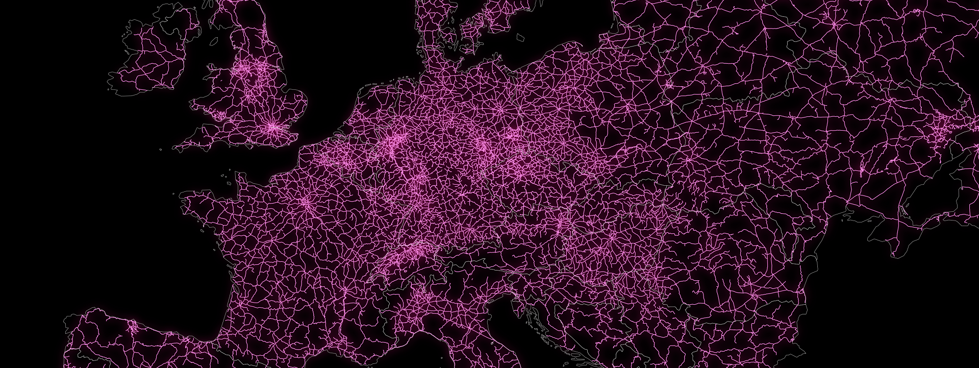
This time we’ll apply the glowing filter to our lines using with_outer_glow. We wrap it around geom_sf and define two colors: one for the line and the other for the glow. Then we define sigma, which is the measure of blurriness of the line in pixels. The higher the sigma, the stronger the glow effect will be. Btw, you could simultaneously apply with_inner_glow to your map to make it shine even brighter!
get_railway_map <- function(p, bb) {

        bb <- get_bounding_box()

        p <- ggplot() +
         with_outer_glow(
                geom_sf(data=rails, color="#FF8DE9", size=0.1, fill=NA),
                colour="#FF1493", sigma=15) +
         geom_sf(data=europe, color="grey80", size=0.05, fill=NA) +
         coord_sf(crs = crsLAEA,
             xlim = c(bb["xmin"], bb["xmax"]),
             ylim = c(bb["ymin"], bb["ymax"])) +
         theme_minimal() +
         theme(
         axis.line = element_blank(),
         axis.text.x = element_blank(),
         axis.text.y = element_blank(),
         axis.ticks = element_blank(),
         axis.title.x = element_text(size=9, color="grey80", hjust=0.25, vjust=3, family = "mono"),
         axis.title.y = element_blank(),
         legend.position = "none",
         panel.grid.major = element_line(color = "black", size = 0.2),
         panel.grid.minor = element_blank(),
         plot.title = element_text(face="bold", size=24, color="grey80", hjust=.5, family = "mono"),
         plot.margin = unit(c(t=1, r=-2, b=-1, l=-2),"lines"),
         plot.background = element_rect(fill = "black", color = NA),
         panel.background = element_rect(fill = "black", color = NA),
         legend.background = element_rect(fill = "black", color = NA),
         panel.border = element_blank()) +
         labs(x = "©2022 Milos Popovic (https://milospopovic.net)\n Data: DIVA-GIS, https://www.diva-gis.org/",
                y = NULL,
                title = "European railways",
                subtitle = "",
                caption = "")

        return(p)
}

p <- get_railway_map()
ggsave(filename="eur_railways.png", width= 8.5, height= 7, dpi = 600, device='png', p)
In the remaining chunk, we add the national boundaries and pass the bounding box.
Look, here is our map! 🥳

In this tutorial, you’ve learned how to load multiple shapefiles and make a pretty railway map of Europe. And we achieved that programmatically in R! Feel free to check the full code here, clone the repo and reproduce, reuse and modify the code as you see fit.
Using this code you can create your own national railway maps! You just need to insert the country name in the download and fetching Europe shapefile sections! Give it a try and let me know how it goes!
I’d be happy to hear your view on how this map could be improved or extended to other geographic realms. To do so, please follow me on Twitter, Instagram or Facebook! Also, feel free to support my work by buying me a coffee here!
