
How to make a neat choropleth map using R
May 15, 2021 | Milos Popovic
In this post, I’ll show you how to make your own choropleth map in R using <200 lines of code. Building on several years of map-making experience, I’ll demonstrate the use of eurostat package to fetch a dataset from Eurostat’s website, download Eurostat’s shapefiles and put everything together in a neat chropleth map. The advantage of this example is that it will allow you to make any map from using the Eurostat data.
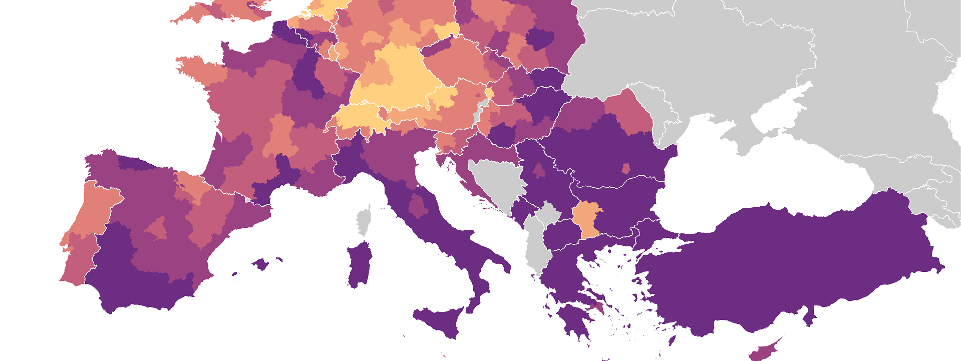
Let’s begin! We’ll use the 2019 Eurostat dataset on young people neither in employment nor in education and training (NEET) by NUTS-2 regions. Following Eurostat, NEETs are individuals who are unemployed or inactive (according to the International Labour Organisation standards) and they haven’t received any formal or non-formal education or training in the four weeks preceding the survey. We’ll map the percentage of the young people aged 15-29 who were NEETs in 2019. Along with the indicators on early leavers from education and training and unempployment, the NEET rate is one of the super important measures for understanding the overall economic perspective of the young population.
We’ll begin by loading several standard libraries for data processing (dplyr), spatial analysis (rgdal and rgeos) and plotting (ggplot2). Also, package classInt will help us construct a discrete measure of the NEET rate. Finally, we’ll use eurostat library to import the dataset into R.
#load libraries
library(ggplot2, quietly=T)
library(rgdal, quietly=T)
library(rgeos, quietly=T)
library(dplyr, quietly=T)
library(classInt, quietly=T)
library(eurostat, quietly=T)
The shapefiles come from Eurostat and include NUTS-2 and country borders that we’ll plot on the map. Now, a few words about NUTS: it’s not what you think 😊! NUTS stands for the Nomenclature of Territorial Units for Statistics. As it name states, NUTS is a geocode for labeling the substate division of countries for statistical purposes. This means that NUTS doesn’t necessarily follow the official national substate divisions. To add more to your confusion, NUTS is developed and regulated by the European Union (EU) so you’ll notice that the data cover the EU members, European Economic Area (Iceland, Norway and Switzerland) and EU candidate countries. That’s why you’ll often see Turkey (EU candidate country) but not Ukraine or Belarus in the maps based on Eurostat data.
Now back to coding. We’ll download and unzip both shapefiles from the Eurostat website. First, let’s download the NUTS regions (the 2016 version) folloeed by the national boundaries (the 2013 version) from the GISCO services website to your working directory.
#download Eurostat NUTS 2016 shapefiles
url <- "https://gisco-services.ec.europa.eu/distribution/v2/nuts/download/ref-nuts-2016-01m.shp.zip" # location on the Eurostat website
download.file(url, basename(url), mode="wb") #download Eurostat country shapefiles
unzip("ref-nuts-2016-01m.shp.zip") # unzip the boundary data
unzip("NUTS_RG_01M_2016_4326_LEVL_2.shp.zip") # unzip the NUTS-2 folder

#download the country shp
url <- "https://gisco-services.ec.europa.eu/distribution/v2/countries/download/ref-countries-2013-01m.shp.zip" # location on the Eurostat website
download.file(url, basename(url), mode="wb") #download Eurostat country shapefiles
unzip("ref-countries-2013-01m.shp.zip") # unzip the boundary data
unzip("CNTR_RG_01M_2013_4326.shp.zip")
Next, we load the shapefiles into R.
#load NUTS shapefile
nuts2 <- readOGR(getwd(),
		 "NUTS_RG_01M_2016_4326_LEVL_2",
		 verbose = TRUE,
		 stringsAsFactors = FALSE)

#load country shapefile
cntry <- readOGR(getwd(),
		 "CNTR_RG_01M_2013_4326",
		 verbose = TRUE,
		 stringsAsFactors = FALSE)
If you run plot(cntry) you’ll notice that Eurostat’s country shapefile covers the whole world. Unfortunately, the shapefile has no column indicating the continent so in order to plot Europe we’ll have to create a bounding box and filter out the remaining African and Asian countries. We’ll first remove those countries and create a bounding box later in ggplot2.
#only European countries on the map
out <- c("MA", "TN", "DZ", "EG", "LY",
	"JO", "IL", "PS", "SY", "SA",
	"LB", "IQ", "IR", "GL")
cn <- subset(cntry, !FID%in%out)
c <- fortify(cn) #turn the SpatialPolygonsDataFrame into data.frame for plotting
Before we download our dataset using the powerful eurostat package I’ll show you how to view the full list of available Eurostat datasets and filtering only NUTS-2 level datasets. The line toc <- eurostat::get_eurostat_toc() returns a data frame stored in our object toc which you could manually inspect by calling fix(toc). If you are, for example, interested in only NUTS-2 level datasets we’ll create an object “k”, assign a string ‘NUTS 2’ and then use this string to filter the title column in our toc dataframe to return only titles that include NUTS 2. Pretty cool, huh?
# search for datasets on NUTS 2 level in their title
toc <- eurostat::get_eurostat_toc()
k <- 'NUTS 2'
t <- subset(toc, grepl(k, title))
In the following chunk, we’ll select the NEET rate dataset (“edat_lfse_22”).
# get NUTS2-level data on NEET rate
edat_lfse_22 <- eurostat::get_eurostat("edat_lfse_22",
                                    time_format = "num")
Also, we’ll select the most recent year (i.e. 2019) for our project. When it comes to the age range there are a few options available (ages 15-24, 15-29, and 18-24). Naturally, I’d choose the 18-24 age bracket because legal age is one of the main requirements to be employed in some EU countries even if we ignore the possibility that some young people may pursue bachelors degree in their early twenties. However, given that the NEET definition takes into account either employment or education or training of the participants we might just go for a wider age range, i.e. 15-29. Another reason for ditching 18-24 in favor of 15-29 is that the former has far more missing values. So, we’ll go for the 15-29 threshold for the sake of having a more complete product. Additionally, we’ll set sex==“T”, meaning that we consider the total NEET rate; other options include values for females (“F”) and males (“M”), which may come in handy when you are interested in plotting gender differences. Finally, we only need the NUTS geocode (“geo”) and the NEET rate (“values”). We’ll rename “geo” to “NUTS_ID” to be able to merge the dataframe with our spatial object “nuts2”.
# let's subset the dataset
neet <- edat_lfse_22  %>%
  			filter(time==2019, # only the year of 2019
				       age=="Y15-29", # ages 15-29
				       sex=="T") %>% # all genders
    		dplyr::select (geo, values)
names(neet)[1] <- "NUTS_ID"
The time is ripe to merge our dataframe with the shapefile and return the new object in the form of dataframe to be plotted in ggplot2.
# merge shp and data.frame
f1 <- merge(neet, nuts2, by="NUTS_ID")
e <- fortify(nuts2, region = "NUTS_ID") %>%
  mutate(NUTS_ID = as.character(id))
d <- e %>% left_join(f1, by = "NUTS_ID")
I prefer a discrete to continuous scale for our NEET rate measure because it’s much easier to distinguish among the colors when you have clear-cut categories and labels. The following chunk of code originates from Timo Grossenbacher’s fantastic post on how to make a choropleth map of Switzerland.
Following Timo’s code, we’ll first compute the natural interval of our measure using quantile breaks to get our cutpoints. I usually stick to 6-8 cutpoints to keep the colors discernible.
# let's find a natural interval with quantile breaks
ni = classIntervals(d$values,
	            n = 6,
	            style = 'quantile')$brks
Then we’ll create labels based on the above cutpoints and round them to get rid of the decimals.
# this function uses above intervals to create categories
labels <- c()
for(i in 1:length(ni)){
    labels <- c(labels, paste0(round(ni[i], 0),
                             "–",
                             round(ni[i + 1], 0)))
}
labels <- labels[1:length(labels)-1]
Finally, let’s carve out the categorical variable (“cat”) based on the cutpoints.
d$cat <- cut(d$values,
              breaks = ni,
              labels = labels,
              include.lowest = T)
levels(d$cat) # let's check how many levels it has (6)
Ah, one more thing that I’d add to Timo’s excellent code: because we have missing values we’ll create an additional category labeled “No data”.
# label NAs, too
lvl <- levels(d$cat)
lvl[length(lvl) + 1] <- "No data"
d$cat <- factor(d$cat, levels = lvl)
d$cat[is.na(d$cat)] <- "No data"
levels(d$cat)
We are ready to plot (finally 🙄)! First things first, we’ll plot the NEET rate regional distribution and overlay it with country borders. The geom_polygon argument will fill in the polygons while the geom_path will draw the national and regional lines. We start off with national polygons followed by NUTS polygons. You’ll notice that I use subset(d, !is.na(values)) to get rid of the NUTS polygons with missing values. In order to fill the missing country/regional polygons with gray, we set fill = “grey80” in the geom_polygon argument for the overlaying national polygons. This will ensure that no country or region is blank. Also, this order of appearance makes sure that only missing polygons are assigned the NA color (“grey80”).
Then, ggplot2 will draw the regional lines and national borders. Usually I assign color=NA and size=0 to the geom_path argument responsible for drawing the NUTS regional boundaries to avoid multiple lines on the map.
p <-
ggplot() +
geom_polygon(data = c, aes(x = long,
                            y = lat,
                            group = group),
                  fill = "grey80") +
geom_polygon(data = subset(d, !is.na(values)), aes(x = long,
                                y = lat,
                                group = group,
                  fill = cat)) +
geom_path(data = subset(d, !is.na(values)), aes(x = long,
                                   y = lat,
                                   group = group),
              color = NA, size = 0) +
geom_path(data = c, aes(x = long,
                                   y = lat,
                                   group = group),
              color = "white", size = 0.2)
When making the map of Europe I like to use the Lambert projection as it gives the continent a more elegant look than the default mercator projection. Here, we’ll also set a bounding box for Europe to make the plot focus on the old continent and assign longitude (xlim) and latitude (ylim) bounds to our map.
p1 <- p + coord_map(xlim=c(-10.6600,44.07), ylim=c(32.5000,71.0500), projection="lambert", parameters=c(10.44,52.775)) +
expand_limits(x=c$long,y=c$lat)
Don’t forget to include your title and/or subtitle, the source of your data and the name of the map creator 😉.
p2 <- p1 + labs(x = "",
     title="Young people aged 25-34 not in\neducation, employment or training in 2019",
     subtitle = "NUTS-2 level",
     caption="©2021 Milos Popovic https://milospopovic.net\nSource: Eurostat\nhttps://appsso.eurostat.ec.europa.eu/nui/show.do?dataset=edat_lfse_38&lang=en")
We’ll assign a manual color palette to our scheme and I like to use Adobe Color to mix the colors and then filter them through Chroma.js Color Palette Helper to determine if the palette is colorblind friendly. We’ll also modify the last numeric label to indicate that it encompasses all the values higher than 15. I like the horizontal legend because it’s more intuitive and visible at the bottom or top of the graph. Also, let’s make the keywidth a bit longer to accommodate every label and, thiner, to give the legend a more elegant look.
p3 <- p2 + scale_fill_manual(name= "% of population aged 15-29",
  values=c('#ffd080', '#f4a77a', '#e18079', '#c35e7d', '#9b4283', '#6c2d83', "grey80"),
  labels=c("4–6",     "6–7",     "7–10",    "10–12",   "12–15",   ">15",   "No data"),
  drop=F)+
guides(fill=guide_legend(
            direction = "horizontal",
            keyheight = unit(1.15, units = "mm"),
            keywidth = unit(15, units = "mm"),
            title.position = 'top',
            title.hjust = 0.5,
            label.hjust = .5,
            nrow = 1,
            byrow = T,
            reverse = F,
            label.position = "bottom"
          )
    )
We’ll wrap up this project with a set of options for the plot background, legend, (sub)title color and size as well as margins. We’ll set a white background to put our map into the focus. I like to choose a colorful title and subtitle that match the legend colors and push them down so that they are visible when you post them on social media. The legend is slighlty centered and placed at the bottom of the plot while the caption is in light gray and below the legend. I like to keep it present but discrete. Finally, plot.margin values are set to negative values to cut any remaining white space on any side of the plot. It’s a very conveninent option if you don’t won’t to cut your map in paint.
p4 <- p3 + theme_minimal() +
theme(panel.background = element_blank(),
legend.background = element_blank(),
legend.position = c(.45, .04),
panel.border = element_blank(),
panel.grid.minor = element_blank(),
panel.grid.major = element_line(color = "white", size = 0),
plot.title = element_text(size=20, color="#6c2d83", hjust=0.5, vjust=-10),
plot.subtitle = element_text(size=14, color="#bd5288", hjust=0.5, vjust=-15, face="bold"),
plot.caption = element_text(size=9, color="grey60", hjust=0.5, vjust=9),
axis.title.x = element_text(size=7, color="grey60", hjust=0.5, vjust=5),
legend.text = element_text(size=10, color="grey20"),
legend.title = element_text(size=11, color="grey20"),
strip.text = element_text(size=12),
plot.margin = unit(c(t=-2, r=-2, b=-2, l=-2),"lines"), #added these narrower margins to enlarge map
axis.title.y = element_blank(),
axis.ticks = element_blank(),
axis.text.x = element_blank(),
axis.text.y = element_blank())
That would be all folks! I really hope this example will help you launch your own mapping project. Feel free to check the full code here, clone the repo and reproduce, reuse and modify the code as you see fit. The advantage of this code is that it allows you to produce maps using any Eurostat dataset directly from R instead of manually downloading the data. However, there are alternative ways of plotting this choropleth map and I’ll make another post on how to use the sf package together with ggplot2 to effortlessly make your own map.
I’d be happy to hear your view on how this map could be improved or extended to other geographic realms. To do so, please follow me on Twitter, Instagram or Facebook!