Geospatial Business Intelligence 101: Computing the shortest driving distance using R
June 22, 2021 | Milos Popovic
When marketing a business, one of the things to keep in mind is how far you should extend your catchment area for attracting new customers. If you are a small business owner, you are likely to lack the resources to cast your net wide. So, it’s very important to identify areas with low competitive intensity. Imagine a petroleum company plans to open multiple gasoline stations across a capital city of a country and you were hired to conduct business intelligence of competitor branch networks within a service area. What do you do? You could, for instance, analyze the density of rival stores per square kilometer for every inhabited area. Another elegant solution covered in this tutorial is to analyze the shortest driving distance of potential customers to the nearest existing petrol stations.
In this post, we’ll tap into the basics of Geospatial Business Intelligence (GeoBI) to explore the competitive position of petrol stations using the case of Belgrade (Serbia). You’ll learn how to calculate the shortest driving distance from every locality to a petrol station using no more than 200 lines of code in R. This tutorial will equip you with the skills necessary to conduct your own competition analysis on, for example, food, and grocery retail, sport and entertainment or the hospitality industry. Such GeoBI reports could ultimately help your clients gain a competitive advantage in their respective industries. Awesome 😮!
We’ll kick off our journey with the help of OpenStreetMaps data that includes the shapefiles on the roads and petroleum stations in Belgrade. Then we’ll import the 2021 official Serbian census boundary data generously brough to us by the one and only Justin Elliot Meyers. Finally, we’ll use package dodgr to compute the driving distance from the centroid of every census locality in Belgrade to the nearest petrol station via driving roads. We’ll wrap up this demo with a cool choropleth map of Belgrade.
Let’s start off by loading the collection of packages for data processing via tidyverse; the osmdata library for importing the OSM data via the Overpass API; and sf for dealing with spatial vector files. Most importantly, we’ll use dodgr to compute the shortest driving distance from every centroid to a petrol station, and geosphere to compute shortest aerial distance in a few cases where it is impossible to calculate the driving distance. Finally, we’ll use ggmap to create a quick and dirty map of Belgrade’s roads and petrol stations R as well as classInt to make the discrete values for our map legend and extrafont to load my favorite Georgia font.
if(!require("tidyverse")) install.packages("tidyverse")
if(!require("osmdata")) install.packages("osmdata")
if(!require("sf")) install.packages("sf")
if(!require("dodgr")) remotes::install_git("https://git.sr.ht/~mpadge/dodgr")
if(!require("geosphere")) install.packages("geosphere")
if(!require("classInt")) install.packages("classInt")
if(!require("extrafont")) install.packages("extrafont")
if(!require("ggmap")) install.packages("ggmap")

library(tidyverse, quietly=T) # data processing
library(osmdata, quietly=T) # load osm data
library(sf, quietly=T) # use spatial vector data
library(dodgr, quietly=T) # driving distance
library(geosphere, quietly=T) # aerial distance
library(classInt, quietly=T) # legend
library(extrafont, quietly=T) # font

set.seed(20210618)
Let’s get this party started by downloading the Serbian census circles from Justin’s GitHub repo and importing the files as sf object. A census circle is the lowest level of analysis in the Serbian geographic framework and every circle consists of approximately 130 households of varying geographic size. This file comes in WGS84/UTM zone 34N coordinate reference system, which we’ll convert into a standard WGS84/EPSG:4326 format.
#download official 2021 Serbian census circles
u <- "https://github.com/justinelliotmeyers/Official_Serbia_2021_Administrative_Boundaries/raw/main/popisni_krug-gpkg.zip"
download.file(u, basename(u), mode="wb")
unzip("popisni_krug-gpkg.zip")

#load census circles
pk <- st_read(paste0(getwd(), "/tmp/data/ready/pk/", "popisni_krug.gpkg"), stringsAsFactors = FALSE) %>%
        st_transform(4326) %>%
        st_as_sf()
In this tutorial, we only need the Belgrade census circles, but filtering them directly from the shapefile is not straightforward because there is no unique identifier that separates the Serbian capital from the rest. So, our next best option is to clip the polygons by Belgrade’s bounding box. To do so, we first import a georeferenced map of Belgrade using ggmap::get_map. We then extract the minimum and maximum latitude and longitude coordinates, which are stored in bg_map under an attribute labeled bb (an acronym for bounding box). Finally, we store the coordinates into our bbox.
# define Belgrade's bounding box based on ggmap's bounding box
bg_map <- ggmap::get_map(getbb("Belgrade"),
	maptype = "toner-lite",
	source = "stamen",
	color="bw",
	force=T)

bg_bbox <- attr(bg_map, 'bb')

bbox <- c(xmin=bg_bbox[,2],
	ymin= bg_bbox[,1],
	xmax= bg_bbox[,4],
	ymax=bg_bbox[,3])

#filter Belgrade
pkb <- st_crop(pk, bbox)
plot(pkb["objectid"])
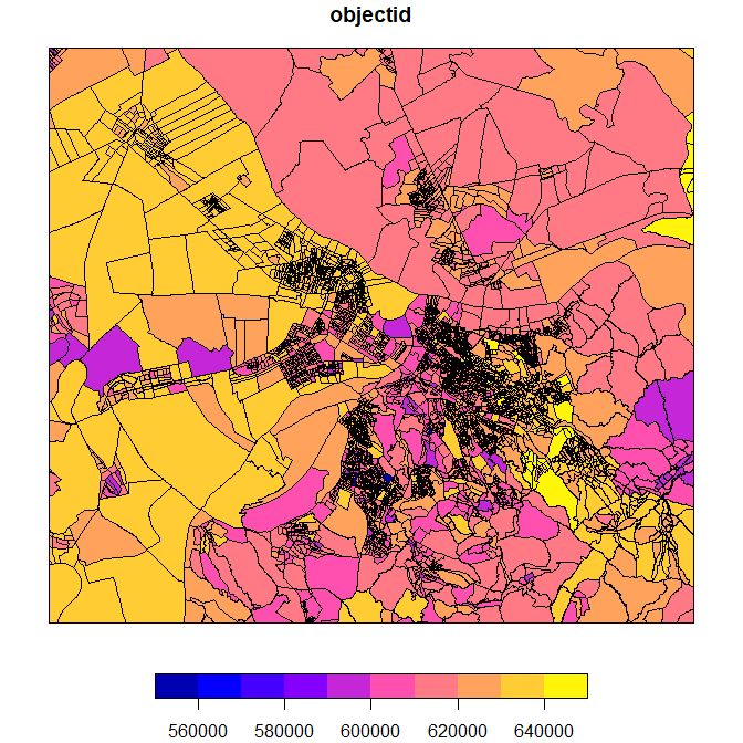
Now we can clip the pk file by bbox using st_crop and obtain our Belgrade census circles. Let’s plot our newborn by calling plot(pkb[“objectid”]). Voila! Below is the clipped vector file of 5,912 Belgrade’s census circles that we’ll use to compute centroids for every circle.
Speaking of which, we use centroids because they are in the form of points, which allows us to compute their distance to petrol stations which are also in the form of points. The following chunk creates the desired centroids for every Belgrade census circle with the help from st_centroid.
#create centroids and their unique identifier
cen <- st_centroid(pkb)
cen$id <- 1:max(nrow(cen))
Next, we’ll load the petrol stations from the OSM data. We’ll make sure that we load only petrol stations using add_osm_feature(key = ‘amenity’, value = “fuel”) and that these stations fall within our pre-defined Belgrade bounding box by specifying bbox = bbox. This returns a list of points and a few polygons. Since we are solely interested in the geolocations we filter out the polygons from the bg_pts list. To put a cherry on top, we elegantly transform this list into an sf object through do.call(rbind, bg_pts). Our bg_p object includes a unique identifier and coordinates for every petrol station.
#fetch Belgrade's petrol stations
bg_amen <- opq(bbox = bbox, timeout = 180, memsize = 104857600) %>%
      add_osm_feature(
      key = 'amenity',
      value = "fuel"
    ) %>%
  osmdata_sf(quiet = FALSE)

bg_pts <- bg_amen[c("osm_points")] #filter only points
bg_p <-  do.call(rbind, bg_pts) %>% #turn from list to sf object
		  select("osm_id", "geometry")
Next we run a similar code to obtain driving roads through the following chunk.
#get Belgrade's paved roads
bg_way <- opq(bbox = bbox, timeout = 120, memsize = 104857600) %>%
      add_osm_feature(
      key = 'highway') %>%
  osmdata_sf(quiet = T)

bg_r <- bg_way$osm_lines
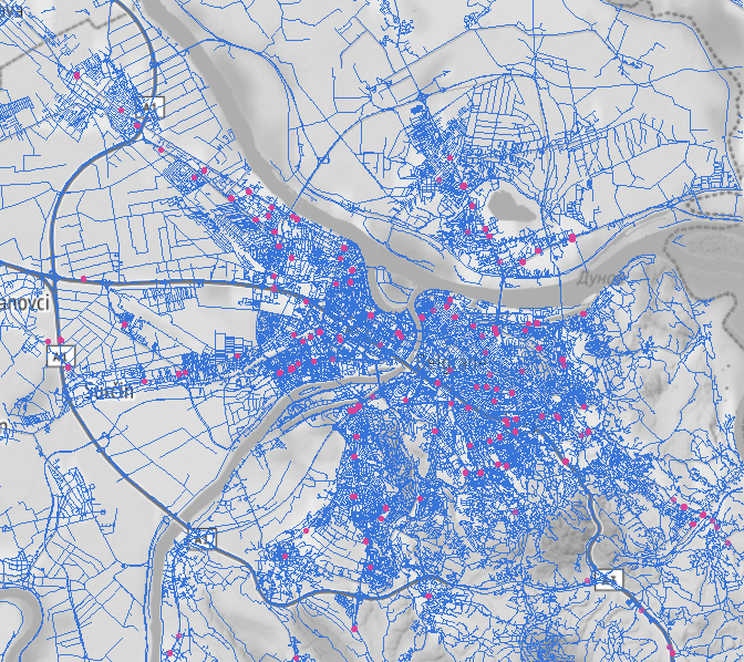
Let’s check if we took that left turn at Albuquerque to end up in Belgrade 😋. The code below will plot Belgrade’s landscape, driving roads (blue) and petrol stations (pink).
# let's peek into the locations of ATMs/banks and roads
ggmap::ggmap(bg_map)+
  geom_sf(data = bg_r,
          inherit.aes = F,
          col = "#3875D9",
          size = .15)+
  geom_sf(data = bg_p,
          inherit.aes = F,
          col = "#d94496",
          alpha = .6,
          size = 1.5)+
  theme_void()
Let’s get our hands dirty with GeoBI, shall we? As mentioned above, we’ll use package dodgr to compute the shortest driving distance. This package allows us to produce dual-weighted computations of distance as it takes into account both the type of way and mode of transport. In other words, the resulting distance will vary if you, for example, drive on a motorway versus a residential street as well as if you cycle versus walk. Another cool thing about this package is that it calculates the shortest many-to-many routing option faster than equivalent packages even in large routing tasks.
Using function weight_streetnet we set motorcar as our preferable mode of transport and different types of highways to be used for weighting. Then we decompose our roads into unique vertices with info on distinct id for every vertice (edge_id), coordinates (from_lon, from_lat, to_lon, to_lat) as well as distance and time weights (d_weighted, time_weighted). This information is stored in our newly created object g.
g <- weight_streetnet(bg_r, wt_profile = "motorcar", type_col = "highway")
dim(g)
head(g)
Next we need to turn our centroids and station locations into coordinates. The centroids will be our origin (from) and the stations will be our destination (to). We then run function dodgr_dists that will calculate the matrix of pair-wise distances between the centroids and petrol stations via a double-weighted network of highways. The resulting matrix includes info on all possible distances (in meters) and we use apply(d, 1, FUN=min, na.rm=TRUE) to filter only the shortest distance for every row. Finally, we merge these distances with our Belgrade census circles and rename the distance column to dist.
# define origin, destination and compute distance
from <- st_coordinates(cen)
to <- st_coordinates(bg_p)
d <- dodgr_dists(graph = g, from = from, to = to)
df <- apply(d, 1, FUN=min, na.rm=TRUE) %>% as.data.frame()
b <- st_sf(data.frame(pkb, df))
names(b)[14] <- "dist"
You may have noticed that the output returned 44 warnings. Upon a closer inspection, we noticed that the function calculated infinite distances for 44 centroids (0.7%). This means that the driving road from these centroids may not be connected with any existing petrol station.
summary(b$dist)
nrow(subset(b, dist=="Inf"))
Do not despair, my friend. We’ll calculate the aerial distance instead. To do so, we need to assign a unique key to every census circle in our spatial data and subset those where the distance to the destination is infinite. Then we’ll use this info to filter those centroids with infinite values and turn them into coordinates. Finally, we need to turn this object into a data frame.
# calculate the aerial distance from every centroid to the closest station
b$id <- 1:max(nrow(b)) # create id
binf <- subset(b, dist=="Inf") #subset rows with infinite values
cinf <- subset(cen, id%in%binf$id) #filter coords by rows with infinite values
c <- st_coordinates(cinf) # get coordinates
c <- as.data.frame(cbind(c, cinf$id)) #convert into df
names(c) <- c("long", "lat", "id") #choose intuitive names
In the following chunk, we create a function that uses distGeo from library geosphere to calculate the shortest aerial path between two points. In our case, we need the minimal distance between every centroid (“sd”) and station (“to”). We obtain dist_mat data frame by applying our newly minted function to our centroids.
# function to find the shortest aerial distance
min_dist <- function(loc){
 sd <- c[c$id==loc,]
 sd1 <- distGeo(sd[,1:2], to[,1:2])
 sd2 <- data.frame(id = loc,
 				   dist=min(sd1))
 return(sd2)
}
dist_mat <- dplyr::bind_rows(lapply(c$id, min_dist))
In the final step, we replace the infinite values with new distance values.
# plug new distances back into "b" and create "bb"
# use if_else to replace infinite values with aerial distance
bb <- b %>%
  left_join(dist_mat, by = "id") %>%
  mutate(dist = if_else(is.infinite(dist.x), dist.y, dist.x))
We are almost ready for mapping! Using our old friend, package classInt we’ll find a natural interval of our distance values and create 8 labels based on the cutpoints.
# let's find a natural interval with quantile breaks
ni = classIntervals(bb$dist,
           n = 8,
           style = 'quantile')$brks

# this function uses above intervals to create categories
labels <- c()
for(i in 1:length(ni)){
    labels <- c(labels, paste0(round(ni[i], 0),
                             "–",
                             round(ni[i + 1], 0)))
}
labels <- labels[1:length(labels)-1]

# finally, carve out the categorical variable based on the breaks and labels
bb$cat <- cut(bb$dist,
              breaks = ni,
              labels = labels,
              include.lowest = T)
levels(bb$cat) # let's check how many levels it has (8)
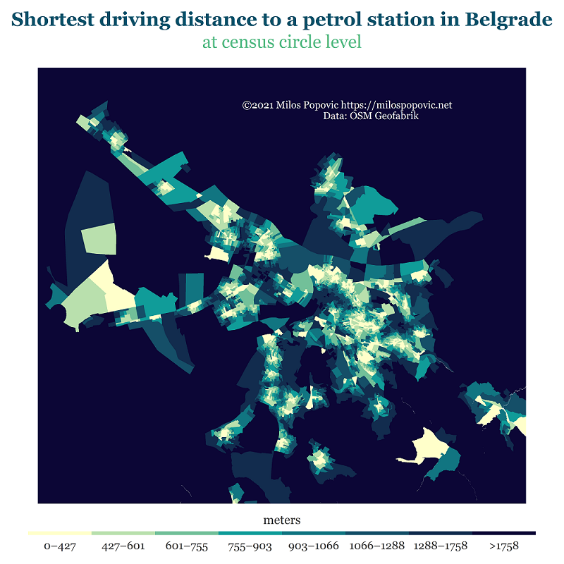
We first plot our distance categories using geom_sf. We’ll remove those Belgrade circle boundaries to keep the map neat and clean while avoiding intensive computation.
Once again, we’ll use colors from Adobe Color and make our palette colorblind friendly with the help of Chroma.js Color Palette Helper. We’ll also modify the last numeric label to indicate that it encompasses all the values higher than 1758 meters.
# plot
p <- ggplot() +
geom_sf(data=bb, aes(fill = cat), color=NA, size=0) +
    coord_sf(crs = 4326, datum = NA) +
  scale_fill_manual(name= "meters",
    		values = c('#ffffca', '#b9e0ad', '#72c099', '#109c99',
    		   '#117581', '#154f68', '#122c4e', '#0c0636'),
    		labels = c("0–427",      "427–601",    "601–755",
    				   "755–903",    "903–1066", "1066–1288",
    				   "1288–1758",  ">1758"),
    		drop = F)+
  guides(fill = guide_legend(
         direction = "horizontal",
         keyheight = unit(1.15, units = "mm"),
         keywidth = unit(20, units = "mm"),
         title.position = 'top',
         title.hjust = 0.5,
         label.hjust = .5,
         nrow = 1,
         byrow = T,
         reverse = F,
         label.position = "bottom"
          )) +
    theme_minimal() +
  theme(text=element_text(family="Georgia"),
    axis.line = element_blank(),
    axis.text.x = element_blank(),
    axis.text.y = element_blank(),
    axis.ticks = element_blank(),
    axis.title.x = element_text(size=9, color="white", hjust=.7, vjust=200),
    axis.title.y = element_blank(),
    legend.position = c(.5, -.015),
    legend.text = element_text(size=10, color="grey20"),
    legend.title = element_text(size=11, color="grey20"),
    panel.grid.major = element_line(color = "white", size = 0.2),
    panel.grid.minor = element_blank(),
    plot.margin     =   unit(c(t=0, r=0, b=0, l=0),"lines"), #added these narrower margins to enlarge map
    plot.title = element_text(face="bold", size=17, color="#095169", hjust=.5, vjust=-2),
    plot.subtitle = element_text(size=16, color="#53ba83", hjust=.5, vjust=-2),
    plot.background = element_rect(fill = "white", color = NA),
    panel.background = element_rect(fill = "white", color = NA),
    legend.background = element_rect(fill = "white", color = NA),
    panel.border = element_blank()) +
  labs(x = "©2021 Milos Popovic https://milospopovic.net\n Data: OSM Geofabrik",
    title = "Shortest driving distance to a petrol station in Belgrade",
    subtitle = "at census circle level",
    caption = "")
Thanks for reading my tutorial on how to carry out basic GeoBI by calculating the shortest driving distance to petrol stations in Belgrade. I really hope that this post will inspire you to carry out similar data analyses. This tutorial could easily be extended to other similar realms to make sense of the market, its key players as well as the customer catchment area. I strongly believe that this and similar projects could help your clients better understand their prospective investment opportunities.
You may ask yourself: OK, but where do I go from here? Well, I got a challenge for you, dear reader. Try to calculate the shortest cycling distance from every building to the closest convenience store or supermarket in The Hague (Netherlands). You could use this official dataset to retrieve the shapefile of all the buildings in the city. You could fetch the locations of convenience stores and supermarkets from OSM data via the osmdata library. Keep in mind that you need to use shop as your key and supermarket and convenience as values:
add_osm_feature(
      key = "shop",
      value = c("supermarket", "convenience")
    )
Feel free to check the full code here, clone the repo and reproduce, reuse and modify the code as you see fit. I trust that you’ll be able to produce lots of cool maps with a slight modification of this code.
I’d be happy to hear your view on how this map could be improved or extended to other geographic realms. To do so, please follow me on Twitter, Instagram or Facebook!


